In-class Exercise 6 - Network

Installing packages

pacman::p_load(jsonlite, tidygraph, ggraph, visNetwork, 
               graphlayouts, ggforce, skimr, tidytext, tidyverse)

Data import

mc3_data <- fromJSON("data/mc3.json")

# Extracting links 

mc3_edges <- as_tibble(mc3_data$links) %>%
  distinct() %>%
  mutate(source = as.character(source), 
         target = as.character(target), 
         type = as.character(type)) %>%
  group_by(source, target, type) %>%
  summarise(weights = n()) %>%
  filter(source != target) %>%
  ungroup()

# convert to character for standardisation
# filter to select out all distinct records, where source and target are different entity

Things to note

# Extracting nodes
mc3_nodes <- as_tibble(mc3_data$nodes)

# Managing the data types 
mc3_nodes <- as_tibble(mc3_data$nodes) %>%
  mutate(country = as.character(country), 
         id = as.character(id), 
         ProductServices = as.character(ProductServices), 
         revenue = as.numeric(as.character(revenue)), 
         type = as.character(type)) %>%
  select(id, country, type, revenue, ProductServices)

Ensuring node and links are consistent naming - Extract out nodes from the edges to ensure consistency

id1 <- mc3_edges %>%
  select(source) %>%
  rename(id = source)

id2 <- mc3_edges %>%
  select(target) %>% 
  rename(id = target)

mc3_nodes1 <- rbind(id1, id2) %>%   
  distinct() %>%   
  left_join(mc3_nodes, by = c("id" = "id")) %>%   
  mutate(unmatched = "drop")
  
#doing left join to match, drop everything else that cannot be matched

mc3_graph <- tbl_graph(nodes = mc3_nodes1, 
                       edges = mc3_edges, 
                       directed = FALSE) %>%
  mutate(betweenness_centrality = centrality_betweenness(), 
         closeness_centrality = centrality_closeness())

# displayig graph model
View(mc3_graph)

## trimming the graph with 100,000 vs 300,000
## modify with the network statistics - Filter 

mc3_graph %>%
  filter(betweenness_centrality >= 100000) %>%
  ggraph(layout = "fr") +
  geom_edge_link(aes(alpha = 0.5)) +
  geom_node_point(aes(size = betweenness_centrality, color = "lightblue", 
                      alpha = 0.5)) +
  scale_size_continuous(range = c(1, 10)) +
  theme_graph()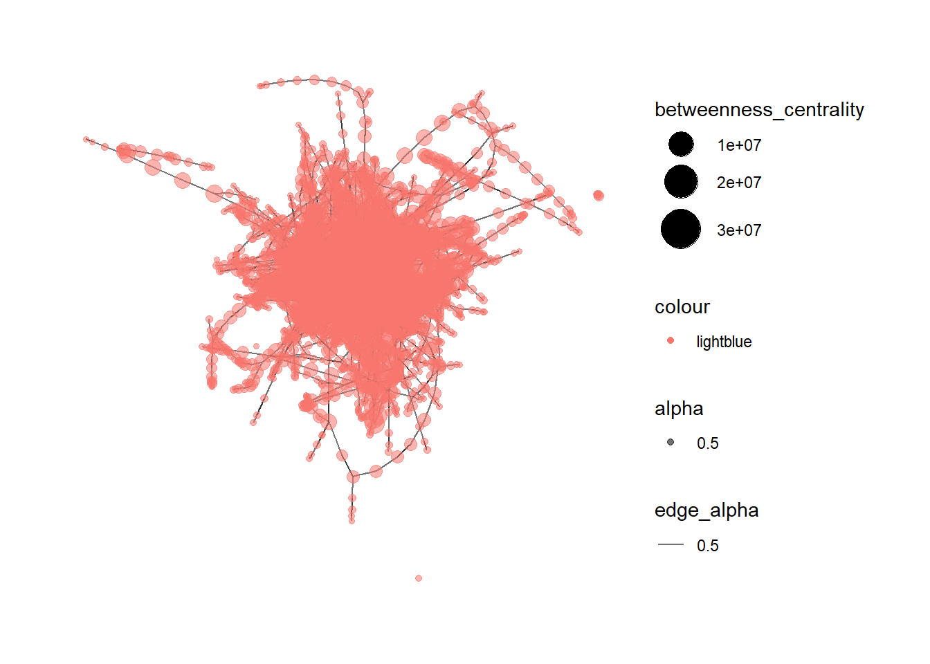

# considering bigger centrality 
mc3_graph %>%
  filter(betweenness_centrality >= 3000000) %>%
  ggraph(layout = "fr") +
  geom_edge_link(aes(alpha = 0.5)) +
  geom_node_point(aes(size = betweenness_centrality, color = "lightblue", 
                      alpha = 0.5)) +
  scale_size_continuous(range = c(1, 10)) +
  theme_graph()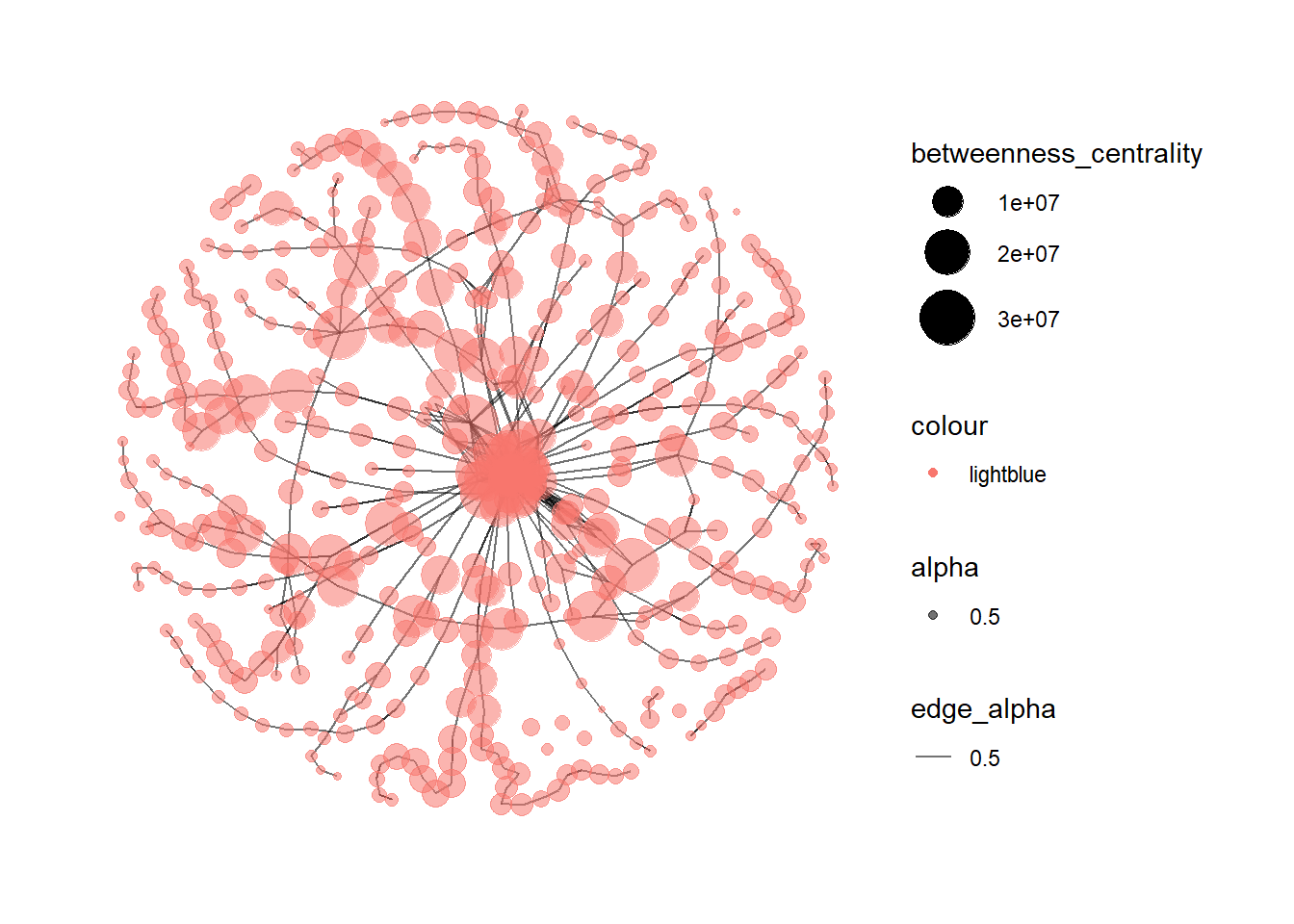

Exploring the nodes data frame

In the cod chunk below,