Take-home Exercise 3 - MC2 Sub Qn 1 & 4

1. Recap of Sub qn 1 & 4

FishEye analysts need help to perform geographic and temporal analysis of the CatchNet data so they can prevent illegal fishing from happening again.

1.1 Approach for Sub qn 1

Goal: Visualisation system to associate vessels with probable cargos.

Steps:

1. Testing various methods to match cargo to vessels (Fishing & Cargo) to identify most robust method.
2. Interactive visualisation of cargo to probable vessels and routes taken
3. Insights from visualisation of seasonality of cargo and anomalities in port exit records.

1.2 Approach for Sub qn 4

Goal: Demonstrate how fishing activity has changed after South Seafood Express Corp was caught.

Steps:

1. Identify date where South Seafood Express Corp was caught based on last seen activity by “Transponder Ping”
2. Comparing median dwell time of fishing vessels per area before and after South Seafood Express (SSE) was caught.
3. Comparing cargo transactions before and after SSE was caught.

2. Data Import and Processing

2.1. Import packages

# import packages 
pacman::p_load(jsonlite, tidyverse, tidyr, 
               knitr, lubridate, dplyr, 
               igraph, ggraph, ggdist, ggplot2, 
               SmartEDA, sf, tidygraph, reshape2, readr,
               DT, patchwork,plotly)

# import relevant datasets

tx_qty <- read_csv("data/tx_qty.csv")
ping_activity <- read_csv("data/ping_activity.csv")
E_Hbrpt_v <- read_csv("data/hbrpt.csv")
N_vessel <- read_csv("data/N_vessel.csv")
location_legend <- read_csv("data/location_legend.csv")
NL_City <- read_csv("data/NL_City.csv")
vessel_movement <- read_rds("data/rds/vessel_movement_data.rds")
oceanus_geog = st_read("data/Oceanus Geography.geojson") %>% st_transform(crs = 4326)

Reading layer `Oceanus Geography' from data source 
  `C:\sengjingyi\ISSS608\Take-home_Ex\Take-home_Ex03\data\Oceanus Geography.geojson' 
  using driver `GeoJSON'
Simple feature collection with 29 features and 7 fields
Geometry type: GEOMETRY
Dimension:     XY
Bounding box:  xmin: -167.0654 ymin: 38.07452 xmax: -163.2723 ymax: 40.67775
Geodetic CRS:  WGS 84

OceanusLocations <- read_rds("data/rds/OceanusLocations.rds")

# extract coordinates from df
coords <- st_coordinates(OceanusLocations)

# drop geometry columns
OceanusLocations_df <- OceanusLocations %>%
  st_drop_geometry()

# append x and y coordinates into df as columns
OceanusLocations_df$XCOORD <- coords[, "X"]
OceanusLocations_df$YCOORD <- coords[, "Y"]

# tidy df by renaming column 
OceanusLocations_df <- OceanusLocations_df %>%
  select(Name, X.Kind, XCOORD, YCOORD) %>%
  rename(Loc_Type = X.Kind)

# reinstating common variables and key data subsets

vessel_colors <- c("Fishing" = "#00CCCC", 
    "Cargo_Vessel" = "#994C00", 
    "Ferry_Cargo" = "#C0C0C0", 
    "Ferry_Passenger" = "#C0C0C0",
    "Research" = "#C0C0C0",
    "Tour" = "#C0C0C0", 
    "Other" = "#C0C0C0")

kind_colors <- c(
  "Island" = "beige", 
  "Fishing Ground" = "lightblue", 
  "Ecological Preserve" = "lightgreen", 
  "city" = "purple", 
  "buoy" = "blue")


# factoring of area
ping_activity$area <- factor(ping_activity$area, 
                             levels = c("Nav E", "Nav D", "Nav C" , "Nav B", "Nav A" ,
                                        "Nav 3", "Nav 2", "Nav 1", 
                                        "Ghoti Preserve", "Don Limpet Preserve", "Nemo Reef", 
                                        "Cod Table","Tuna Shelf","Wrasse Beds",
                                        "Exit East", 
                                        "City of South Paackland", "City of Paackland","City of Lomark","City of Himark","City of Haacklee","City of Port Grove"))


# filtering for fishing and cargo vessels

fishing_v <- N_vessel %>% filter(vessel_type == "Fishing")
cargo_v <- N_vessel %>% filter(vessel_type == "Cargo_Vessel")

# filtering for fishing vessel activity and cargo vessel activity

fish_v_activity <- ping_activity %>% 
  filter(vessel_id %in% fishing_v$vessel_id)

cargo_v_activity <- ping_activity %>% 
  filter(vessel_id %in% cargo_v$vessel_id)

3. Addressing Mini-challenge 2 - Sub-question 1 of Mapping vessels to cargo.

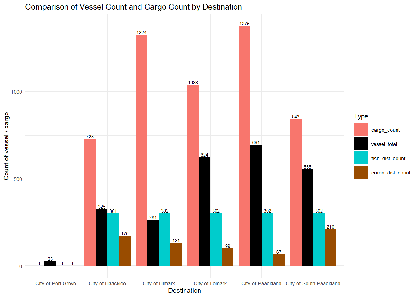
3.1 Preliminary Comparison of Total Count to Vessels (Fishing & Cargo) per port.

Insights derived:

1. Vessels that visit Port Grove is only for Tourism and no cargo delivered. Associated vessel types are not “Fishing” or “Cargo Vessels”. Hence, Port Grove will be excluded from subsequent matching.

2. Within Transponder Ping data set, multiple pings originate from the same vessel_id at same port on the same date, but differing time (hours and minutes) hence, to simplify, we will aggregate the distinct vessel_id and group by same date, same port to minimise duplicates of the same vessel.

3. Substantially larger distinct count of cargo_id to distinct vessel_id. This suggest that 1 vessel may deposit one or more cargo, especially when each cargo only includes 1 fish species. Hence, possible investigation include:

   1. Same vessel delivering multiple cargo of same fish species on the same day to split total volume of fish caught to prevent being flagged for over-fishing,

   2. Same vessel delivering multiple cargo of different fish species on same day, where each cargo is labelled by distinct fish species.

# Comparing entries per port with boxplot

## tx_qty -> Type of species per port 
cargo_count <- tx_qty %>%
  group_by(dest) %>%
  summarize(cargo_count = n())

unique_dest <- unique(cargo_count$dest) # only 5 cities

## count of vessel by port
hb_count <- E_Hbrpt_v %>%
  group_by(port) %>%
  summarize(vessel_total = n()) 

unique_port <- unique(hb_count$port) # 6 cities

## To recalculate based on distinct vessel per day per port. 
fish_dist_p_count <- fish_v_activity %>%
  mutate(date = as.Date(start_time)) %>%
  group_by(area, date) %>%
  summarize(fishv_dist_p_count = n_distinct(vessel_id)) %>%
  filter(area %in% unique_port)

fish_dist_pcount2 <- fish_dist_p_count %>%
  group_by(area) %>%
  summarize(fish_dist_count = n())

## calculate for cargo vessels

cargo_dist_p_count <- cargo_v_activity %>%
  mutate(date = as.Date(start_time)) %>%
  group_by(area, date) %>%
  summarize(cargov_dist_p_count = n_distinct(vessel_id)) %>%
  filter(area %in% unique_port)

cargo_dist_pcount2 <- cargo_dist_p_count %>%
  group_by(area) %>%
  summarize(cargo_dist_count = n())

# merge for plot 
count <- merge(cargo_count, hb_count, by.x = "dest", by.y = "port", all = TRUE)
count <- merge(count, fish_dist_pcount2, by.x = "dest", by.y = "area", all = TRUE)
count <- merge(count, cargo_dist_pcount2, by.x = "dest", by.y = "area", all = TRUE)
count <- count %>% mutate(across(everything(), ~replace_na(., 0)))

count$dest <- factor(
  count$dest, 
  levels = c("City of Port Grove", "City of Haacklee", "City of Himark", 
             "City of Lomark", "City of Paackland", "City of South Paackland")) 

# reshape for plot 
count2 <- count %>%
  gather(key = "type", value = "count", cargo_count, vessel_total, fish_dist_count, cargo_dist_count)

count2$type <- factor(count2$type, levels = c("cargo_count", "vessel_total", "fish_dist_count", "cargo_dist_count"))

# Define color for the plot

type_colors <- c("cargo_count" = "#F8766D", 
                   "vessel_total" = "black", 
                   "fish_dist_count" = "#00CCCC", 
                   "cargo_dist_count" = "#994C00")


# Plot the grouped bar chart with labels
ggplot(count2, aes(x = dest, y = count, fill = type)) +
  geom_bar(stat = "identity", position = "dodge") +
  geom_text(aes(label = count), 
            position = position_dodge(width = 0.9), 
            vjust = -0.25, size = 2) + 
  labs(title = "Comparison of Vessel Count and Cargo Count by Destination",
       x = "Destination",
       y = "Count of vessel / cargo",
       fill = "Type") +
  scale_fill_manual(values = type_colors) +  # Set the custom colors
  theme_minimal(base_size = 8) +
  theme(axis.line = element_line(color = "black"))

3.2. Possible Matching with Vessels

The table below summarise the results of 3 matching methods for fishing vessels:

S/N	Matching Method	% Match	% Mis-match
1	Tx_c (Cargo import) with E_Hbrpt_v (Vessel Harbor Arrival) by date	2454 / 5307 = 46%	307 = 54%
2	Tx_c (Cargo Import) with Ping Activity (Vessel at port) by date	5307 / 5307 = 100%	-
3	Tx_c (Fish Species) with Ping Activity (Past route & probable fishes caught)	4957 / 5003 = 99%	46 / 5003 = 1%

3.2.1 Method 1 - Direct Match of Habor Report of vessel with Cargo Transactions on Port and Date

Limitation: As mentioned in the data description, no harbor reports the vessels everyday, the dataset used of Event.HarborReport might not have the complete depiction of the vessels arrival.

Visualisation:

1. Interactive scatter graph with each dot representing 1 unique cargo_id, across time period of interest by adjustable parameter earliest_date to latest_date.
2. Facet-grid to show the cargo at other ports of the same period
3. Color-coding where Matched cargo records are in green, and unmatched cargos are flagged in red.
4. Tool-tip included to identify which date, which unique cargo_id and the probable vessel list.

# cleaning tx_qty to align date-time to only date 
tx_qty1 <- tx_qty %>% 
  mutate(tx_date = as.Date(tx_date))

m1 <- tx_qty1 %>% left_join(E_Hbrpt_v %>% select(arr_date, port, vessel_id), 
                            by = c("tx_date" = "arr_date", "dest" = "port")) %>%
  group_by(cargo_id, dest, tx_date) %>%
  summarize(probable_vessel = list(vessel_id), .groups = "drop")

m1_full <- m1 %>% left_join(tx_qty1 %>% select(cargo_id, fish_species, qty_tons), by = c("cargo_id")) 
m1_full$color <- ifelse(is.na(m1_full$probable_vessel), "Not Matched", "Matched")
match_codes <- c("Matched" = "#00FF00", "Not Matched" = "#FF0000")

# Plot interactive plot 

library(ggiraph)

# to make it interactive, we will subset into suitable range 
earliest_date = c("2035-03-02")
latest_date = c("2035-05-15")

m1_filtered <- m1_full %>% filter(tx_date >= earliest_date, tx_date <= latest_date)

p1 <- ggplot(data = m1_filtered, 
             aes(x = tx_date, y = qty_tons, fill = color, 
                 text = paste("Date:", tx_date, "<br>",
                              "Cargo ID:", cargo_id, "<br>",
                              "Probable Vessel:", probable_vessel))) + 
  geom_point(size = 3, shape = 21, color = NA) +  # Remove border by setting color to NA
  facet_grid(~ dest) + 
  scale_fill_manual(values = match_codes) + 
  labs(title = "Summary of Cargos Match across date & quantity", 
       x = "Transaction Date", 
       y = "Cargo Quantity (Tons)") 
       # Add facet grid by port

# Convert to plotly and include tooltip
ggplotly(p1, tooltip = "text")

m1_summary <- m1 %>%
  mutate(match_status = ifelse(is.na(probable_vessel), "NA", "Matched")) %>%
  group_by(match_status) %>%
  summarize(count = n()) %>%
  mutate(percentage = (count / sum(count)) * 100)

# santising ping activity to table with unique vessel_id per port per date.

ping_activity_c <- ping_activity %>%
  filter(area %in% unique_port, vessel_type == c("Fishing", "Cargo_Vessel")) %>%
  mutate(start_date = as.Date(start_time)) %>%
  group_by(start_date, area) %>% 
  summarize(probable_vessel = list(unique(vessel_id)), .groups = "drop") 

rm(m1, m1_full, m1_filtered)

3.2.2 Method 2 - Direct Match of Transponder Ping of Fishing Vessels with Cargo Transactions on Port and Date

Limitation: Over-matching due to over-sensitive Transponder pings where fishing vessels may be near the coast but have not disembark to unload cargo, may be matched with existing cargo list.

Visualisation: Repeat the code for Method 1 plot, but now all points are highlighted in “green” due to over-matching.

m2 <- tx_qty1 %>% left_join(ping_activity_c, 
                            by = c("tx_date" = "start_date", "dest" = "area")) %>%
  group_by(cargo_id, dest, tx_date)

m2_full <- m2 %>% left_join(tx_qty1 %>% select(cargo_id, fish_species, qty_tons), by = c("cargo_id")) 
m2_full$color <- ifelse(is.na(m2_full$probable_vessel), "Not Matched", "Matched")
match_codes <- c("Matched" = "#00FF00", "Not Matched" = "#FF0000")

# to make it interactive, we will subset into suitable range 
earliest_date = c("2035-03-02")
latest_date = c("2035-05-15")

m2_filtered <- m2_full %>% filter(tx_date >= earliest_date, tx_date <= latest_date)

p2 <- ggplot(data = m2_filtered, 
             aes(x = tx_date, y = qty_tons.x, fill = color, 
                 text = paste("Date:", tx_date, "<br>",
                              "Cargo ID:", cargo_id, "<br>",
                              "Probable Vessel:", probable_vessel))) + 
  geom_point(size = 3, shape = 21, color = NA) +  # Remove border by setting color to NA
  facet_grid(~ dest) + 
  scale_fill_manual(values = match_codes) + 
  labs(title = "Summary of Cargos Match across date & quantity", 
       x = "Transaction Date", 
       y = "Cargo Quantity (Tons)") 
       # Add facet grid by port

# Convert to plotly and include tooltip
ggplotly(p2, tooltip = "text")

m2_summary <- m2 %>%
  mutate(match_status = ifelse(is.na(probable_vessel), "NA", "Matched")) %>%
  group_by(match_status) %>%
  summarize(count = n()) %>%
  mutate(percentage = (count / sum(count)) * 100)


rm(m2_full, m2, m2_filtered)

3.2.3 Method 3 - Indirect Match based on Routes pieced together by Transponder Ping, and eventual unloading based on Harbor Report.

Data Wrangling:

1. Align the fields of Vessel Harbor Report with Transponder ping activity.
2. Append the 2 data sets to from a combined history of locations visited by the vessel, with an additional column of Report to identify source.
3. Arrange the list of records by vessel_id and start_date to list the possible route taken by each vessel chronologically.
4. Reformat the data structure such that the list of areas visited by vessels are stringed together as route_list, including final destination as final_area.
5. A new trip is registered every time the vessel disembark at a harbor, where Report = “Hbrpt” from Harbor Report, and the route_end date is captured when ends at a harbor, and route_start date is captured each time it leaves a harbor.
6. Based on the matrix of possible fish species present in each region, list down the probable fish species expected to be caught if the vessel visited these regions.

## santising ping activity to focus on fishing and cargo vessels, create new column to assign report type as "transponderping" 

ping_movement <- ping_activity %>%
  filter(vessel_type == c("Fishing", "Cargo_Vessel")) %>%
  mutate(start_date = as.Date(start_time)) %>%
  select( c("start_date", "area", "kind", "Activities", "vessel_id", "fish_species_present", "vessel_type", "vessel_company")) %>%
  mutate(report = "transponderping")

# aligning columns of E_Hbrpt_v with ping movement (need to match activities with N_City, varying activities per city)

port_record <- E_Hbrpt_v %>% 
  left_join(NL_City, by = c("port" = "city_id")) %>%
  mutate(report = "hbrpt", kind = "city", fish_species_present = NA) %>% 
  rename(area = port, 
         start_date = arr_date) %>%
  select(c("start_date", "area", "kind", "Activities", "vessel_id", "fish_species_present", "vessel_type", "vessel_company", "report"))

# merge route movement
route <- bind_rows(ping_movement, port_record)
route <- route %>% arrange(vessel_id, start_date)

# reformat data to parse the possible route taken 
route_data <- route %>%
  group_by(vessel_id) %>%
  mutate(trip_id = cumsum(report == "hbrpt")) %>%
  ungroup()

# Function to process routes for each vessel
process_routes <- function(data) {
  data %>%
    group_by(vessel_id, trip_id) %>%
    summarise(
      route_start = first(start_date[report == "hbrpt"]),
      route_end = last(start_date[report == "hbrpt"]),
      route_list = paste(
        c(first(area[report == "hbrpt"]), 
          unique(area[report == "transponderping"]),
          last(area[report == "hbrpt"])), 
        collapse = ", "
      ),
      probable_fish_species = paste(unique(fish_species_present[report == "transponderping"]), collapse = ", "), 
final_area = last(area[report  == "hbrpt"])
    ) %>%
    ungroup()
}

# Apply the function to the dataset
concatenated_routes <- process_routes(route_data)

# filtering to only focus on routes with expected catch

route_w_catch <- concatenated_routes %>% 
  filter(probable_fish_species != "" & 
  probable_fish_species != "NA")

write_csv(route_w_catch, "data/route_w_catch.csv")

# convert fish species to aligned format

library(stringr)

replacements <- c(
  `Cod/Gadus n.specificatae` = "gadusnspecificatae4ba", 
  `Birdseye/Pisces frigus` = "piscesfrigus900", 
  `Sockfish/Pisces foetida` = "piscesfoetidaae7", 
  `Wrasse/Labridae n.refert` = "labridaenrefert9be", 
  `Beauvoir/Habeas pisces` = "habeaspisces4eb", 
  `Harland/Piscis sapidum` = "piscissapidum9b7", 
  `Tuna/Thunnini n.vera` = "thunnininveradb7", 
  `Offidiaa/Piscis osseus` = "piscisosseusb6d", 
  `Helenaa/Pisces satis` = "piscessatisb87", `NA` = "")

route_w_catch <- route_w_catch %>%
  mutate(probable_fish_species = str_replace_all(probable_fish_species, replacements))

datatable(route_w_catch, 
          options = list(pageLength = 3), filter = "top")

Show 3102550100 entries

Search:

	vessel_id	trip_id	route_start	route_end	route_list	probable_fish_species	final_area
		0 19	2035-02-01T00:00:00.000Z 2035-11-28T00:00:00.000Z	2035-02-01T00:00:00.000Z 2035-11-28T00:00:00.000Z
1	albacoreangler47d	0			NA, Nav 2, Exit East, Cod Table, City of South Paackland, Nav 3, NA	, gadusnspecificatae4ba, piscesfrigus900, habeaspisces4eb
2	albacoreangler47d	1	2035-03-11T00:00:00Z	2035-03-11T00:00:00Z	City of Paackland, Nav 3, Cod Table, City of Paackland	, gadusnspecificatae4ba, piscesfrigus900, habeaspisces4eb	City of Paackland
3	albacoreangler47d	3	2035-03-12T00:00:00Z	2035-03-12T00:00:00Z	City of South Paackland, City of South Paackland, Nav 3, Tuna Shelf, Nav 2, Cod Table, Exit East, Nemo Reef, City of South Paackland	, thunnininveradb7, piscesfrigus900, habeaspisces4eb, piscissapidum9b7, gadusnspecificatae4ba, piscesfrigus900, habeaspisces4eb, labridaenrefert9be, thunnininveradb7, piscesfrigus900, habeaspisces4eb, piscessatisb87	City of South Paackland

Showing 1 to 3 of 1,453 entries

Previous12345…485Next

Matching conditions:

1. For each cargo_id, possible vessels should have matching probable_fish_species based on area visited.
2. Hence, for this condition to be possible, we excluded cargo_ids where fish_species = “oncorhynchusrosea790” as there is no geographical region related.
3. For each cargo_id, possible vessels should have matching route_end date as the tx_date of cargo which has already been adjusted 1 day earlier for the same destination as final area in route list.

However, there is a poor match when directly matching route_end date with tx_date for cargo import date. To consider cases where there is some time lapse to transport cargo off the ship, we considered the following time difference.

• Base case: tx_date = route_end date: 946 matches / 5003 total records ~ Approx: 18% match

• Case 1: tx_date within route_end + 2: Returned 394,120 possible combinations ~ Approx 1 cargo_id to 78 vessels, over-matched.

• Case 2: tx_date within route_end + 1: Returned same 394,120 possible combinations ~ Approx 1 cargo_id to 78 vessels, over-matched.

• Case 3: Best-effort basis where tx_date >= route_end date, returning all records where datediff(tx_date and route_end date) is minimized: Returned 11,513 combinations ~ Approx 1 cargo to 2.3 vessels, and count of distinct cargo_id with unmatched record = 46.

Visualisation:

1. To show the count of cargo with the minimised days difference to return a possible match.
2. For cargo_id with a match that is >7 days, this is deemed to be unreasonable and hence flagged as red.
3. Tooltip on the list of cargo_id for that particular day count is added for further details.

# consider excluding cargo with salmon catch, because not possible to map - remaining 5003
tx_qty_wo_sal <- tx_qty1 %>% filter(fish_species != "oncorhynchusrosea790")

# exact match on date = 2514
 m3 <- tx_qty_wo_sal %>% 
  left_join(route_w_catch, by = c("dest" = "final_area", "tx_date" = "route_end")) %>%   
   filter(grepl(fish_species, probable_fish_species))

# Exploring cargos with no match vessels 

mismatched_cargo_m3 <- anti_join(tx_qty_wo_sal, m3, by = "cargo_id") #4057 returned 

# attempt to match cargo to vessel by location (834060 observations returned) - 788038

m3_wo_date <- tx_qty_wo_sal %>% 
  left_join(route_w_catch, by = c("dest" = "final_area")) %>% filter(grepl(fish_species, probable_fish_species))

#write_csv(m3_wo_date, "data/m3_wo_date.csv")

# doing analysis by time
# +2 days - 394120

m3_filtered_2days <- m3_wo_date %>%
  filter(any(tx_date <= route_end + 2 & tx_date >= route_end)) %>%
  distinct(cargo_id, vessel_id, .keep_all = TRUE) 

# +1 days - 394120

m3_filtered_1days <- m3_wo_date %>%
  filter(any(tx_date <= route_end + 1 & tx_date >= route_end)) %>%
  distinct(cargo_id, vessel_id, .keep_all = TRUE)

# returning records with nearest date - 11513 
nearest_tx_date <- m3_wo_date %>%
  group_by(cargo_id) %>%
  filter(tx_date > route_end) %>%  
  filter(abs(difftime(tx_date, route_end, units = "days")) == min(abs(difftime(tx_date, route_end, units = "days")))) %>%
  ungroup()

# understanding any cargo not mapped - 46 (not sure why, but should have mapping)
mismatched_cargo_nearest_tx <- anti_join(tx_qty_wo_sal, nearest_tx_date, by = "cargo_id")
# unique(mismatched_cargo_nearest_tx$fish_species) #labridaenrefert9be

# understanding average days diff

nearest_tx_date <- nearest_tx_date %>%
  mutate(days_diff = as.numeric(difftime(tx_date, route_end, units = "days")))

# Group by days_diff and count the number of records

days_diff_summary <- nearest_tx_date %>%
  group_by(days_diff) %>%
  summarize(count = n(), cargo_ids = paste(cargo_id, collapse = ", "))

# Create the ggplot object
p3 <- ggplot(days_diff_summary, aes(x = days_diff, y = count, fill = days_diff > 7, text = cargo_ids)) +
  geom_bar(stat = "identity") +
  scale_fill_manual(values = c("FALSE" = "steelblue", "TRUE" = "red")) +
  labs(title = "Count of Records by Difference in Days",
       x = "Difference in Days",
       y = "Count of Records") +
  theme_minimal(base_size = 10) +
  theme(axis.line = element_line(color = "black"), legend.position = "none")

# Convert to plotly and include tooltip
ggplotly(p3, tooltip = "text")

# data table of cargo_id that has not found a match: 

datatable(mismatched_cargo_nearest_tx, 
          options = list(pageLength = 5))

Show 5102550100 entries

Search:

	last_edited_by	date_added	last_edited_date	cargo_id	dest	tx_date	fish_species	qty_tons	deliver_date
1	Olokun Daramola	2035-02-04T00:00:00Z	2035-02-04T00:00:00Z	cargo_2035_24532325	City of Himark	2035-02-03	labridaenrefert9be	51.00000000000001	2035-02-04
2	Junior Shurdlu	2035-02-09T00:00:00Z	2035-02-10T00:00:00Z	cargo_2035_245433f5	City of Himark	2035-02-07	labridaenrefert9be	45	2035-02-08
3	Melinda Manning	2035-02-12T00:00:00Z	2035-02-13T00:00:00Z	cargo_2035_24554063	City of Himark	2035-02-10	labridaenrefert9be	54	2035-02-11
4	Olokun Daramola	2035-02-16T00:00:00Z	2035-02-17T00:00:00Z	cargo_2035_24565818	City of Himark	2035-02-14	labridaenrefert9be	58.5	2035-02-15
5	Jack Inch	2035-02-19T00:00:00Z	2035-02-21T00:00:00Z	cargo_2035_24576d01	City of Himark	2035-02-17	labridaenrefert9be	70.5	2035-02-18

Showing 1 to 5 of 46 entries

Previous12345…10Next

# clean the environment
rm(m3_filtered_1days, m3_wo_date, m3_filtered_2days)

3.3 Putting it together

Caveat: Due to the large size of data, to illustrate the visualisation of cargo to vessel, we will use a subset of the data by month of interest and area of interest. The visualisation can be run similarly for the matched 99% of records based on nearest_tx_date

Adjustable parameters include:

• earliest_time: Start date for period of interest & latest_time: End date for period of interest.

• area_of_interest: To define destination where cargo was received and last visited port of the vessel.

Visualisation Attempts for further work.

1. Attempt to link the 2 heat maps by the highlight key of the same arr_date for vessels and tx_date for cargo transactions.
2. Attempt to separate the overlapping legends with layout

# assign values to the parameter

earliest_date = c("2035-08-01")
latest_date = c("2035-08-31")
area_of_interest = c("City of Himark", "City of Haacklee")

# creating subset of interested cargo transactions
tx_int <- nearest_tx_date %>% filter(tx_date >= earliest_date, tx_date <= latest_date, 
                                     dest == area_of_interest) %>% arrange(dest, tx_date)

cargo_summary <- tx_int %>%
  group_by(dest, tx_date) %>%
  summarize(cargo_count = n_distinct(cargo_id), cargo_ids = paste(cargo_id, collapse = ", "))

# Extract week and weekday for calendar heatmap
cargo_summary <- cargo_summary %>%
  mutate(week = week(as.Date(tx_date)),
         weekday = wday(as.Date(tx_date), label = TRUE, week_start = 1))  # Monday as the start of the week

# Plot the calendar heatmap
p4 <- ggplot(cargo_summary, aes(x = week, y = weekday, fill = cargo_count, text = cargo_ids)) +
  geom_tile(color = "white") +
  facet_wrap(~ year(as.Date(tx_date)) + dest, scales = "free_y") +
  scale_fill_gradient(low = "white", high = "blue") +
  labs(title = "Number of Cargo per Week at Each Harbor",
       x = "Week",
       y = "Weekday",
       fill = "Cargo Count") +
  theme_minimal(base_size = 10) +
  theme(axis.line = element_line(color = "black"))

# Convert to plotly for interactivity and expose cargo_ids
p4 <- ggplotly(p4, tooltip = "text")

# repeat for vessel summary
vessel_summary <- E_Hbrpt_v %>% 
  filter(arr_date >= earliest_date, arr_date <= latest_date, 
                                     port == area_of_interest) %>% 
  group_by(port, arr_date) %>%
  summarize(vessel_count = n_distinct(vessel_id), vessel_ids = paste(vessel_id, collapse = ", "))

# Extract week and weekday for calendar heatmap
vessel_summary <- vessel_summary %>%
  mutate(week = week(as.Date(arr_date)),
         weekday = wday(as.Date(arr_date), label = TRUE, week_start = 1))  # Monday as the start of the week

# Create highlight keys for linking
cargo_summary$key <- as.character(cargo_summary$tx_date)
vessel_summary$key <- as.character(vessel_summary$arr_date)

# Plot the cargo calendar heatmap
p1 <- ggplot(highlight_key(cargo_summary, ~key), aes(x = week, y = weekday, fill = cargo_count, text = cargo_ids)) +
  geom_tile(color = "white") +
  facet_wrap(~ year(as.Date(tx_date)) + dest, scales = "free_y") +
  scale_fill_gradient(low = "palegreen", high = "red", name = "Cargo Count") +
  labs(title = "Number of Cargo per Week at Each Harbor",
       x = "Week",
       y = "Weekday") +
  theme_minimal(base_size = 10) +
  theme(axis.line = element_line(color = "black"))

p1 <- ggplotly(p1, tooltip = "text") %>%
  layout(legend = list(x = 1.05, y = 0.5))

# Plot the vessel calendar heatmap
p2 <- ggplot(highlight_key(vessel_summary, ~key), aes(x = week, y = weekday, fill = vessel_count, text = vessel_ids)) +
  geom_tile(color = "white") +
  facet_wrap(~ year(as.Date(arr_date)) + port, scales = "free_y") +
  scale_fill_gradient(low = "lightblue", high = "blue", name = "Vessel Count") +
  labs(title = "Number of Vessels per Week at Each Harbor",
       x = "Week",
       y = "Weekday") +
  theme_minimal(base_size = 10) +
  theme(axis.line = element_line(color = "black"))

p2 <- ggplotly(p2, tooltip = "text") %>%
  layout(legend = list(x = 1.1, y = 0.5))

# return underlying dataset 
datatable(tx_int, 
          options = list(pageLength = 3), 
          filter = "top")

Show 3102550100 entries

Search:

	last_edited_by	date_added	last_edited_date	cargo_id	dest	tx_date	fish_species	qty_tons	deliver_date	vessel_id	trip_id	route_start	route_end	route_list	probable_fish_species	days_diff
		2035-08-02T00:00:00.000Z 2035-09-03T00:00:00.000Z	2035-08-02T00:00:00.000Z 2035-09-05T00:00:00.000Z			2035-08-01 2035-08-31		-4.125000000000000 87.750000000000000	2035-08-02 2035-09-01		4 8	2035-07-09T00:00:00.000Z 2035-08-24T00:00:00.000Z	2035-07-09T00:00:00.000Z 2035-08-24T00:00:00.000Z			1 28
1	Harvey Janus	2035-08-02T00:00:00Z	2035-08-02T00:00:00Z	cargo_2035_309095f5	City of Haacklee	2035-08-01	piscesfoetidaae7	27.75	2035-08-02	maritimemagnitude2e9	7	2035-07-24T00:00:00Z	2035-07-24T00:00:00Z	City of Haacklee, Nav B, Tuna Shelf, City of South Paackland, Nav 3, Cod Table, City of Haacklee	, thunnininveradb7, piscesfrigus900, habeaspisces4eb, piscissapidum9b7, gadusnspecificatae4ba, piscesfrigus900, habeaspisces4eb	8
2	Jack Inch	2035-08-03T00:00:00Z	2035-08-04T00:00:00Z	cargo_2035_28209177	City of Haacklee	2035-08-02	piscesfrigus900	3	2035-08-03	maritimemagnitude2e9	7	2035-07-24T00:00:00Z	2035-07-24T00:00:00Z	City of Haacklee, Nav B, Tuna Shelf, City of South Paackland, Nav 3, Cod Table, City of Haacklee	, thunnininveradb7, piscesfrigus900, habeaspisces4eb, piscissapidum9b7, gadusnspecificatae4ba, piscesfrigus900, habeaspisces4eb	9
3	Harvey Janus	2035-08-04T00:00:00Z	2035-08-06T00:00:00Z	cargo_2035_29614c5a	City of Haacklee	2035-08-02	habeaspisces4eb	46.75	2035-08-03	maritimemagnitude2e9	7	2035-07-24T00:00:00Z	2035-07-24T00:00:00Z	City of Haacklee, Nav B, Tuna Shelf, City of South Paackland, Nav 3, Cod Table, City of Haacklee	, thunnininveradb7, piscesfrigus900, habeaspisces4eb, piscissapidum9b7, gadusnspecificatae4ba, piscesfrigus900, habeaspisces4eb	9

Showing 1 to 3 of 127 entries

Previous12345…43Next

# Combine plots using subplot and arrange legends
subplot(p1, p2, nrows = 2, margin = 0.05, titleX = TRUE, titleY = TRUE) %>%
  layout(annotations = list(
           list(x = 0.5, y = 1.05, text = "Cargo Count", showarrow = FALSE, xref = 'paper', yref = 'paper'),
           list(x = 0.5, y = 0.45, text = "Vessel Count", showarrow = FALSE, xref = 'paper', yref = 'paper')
         )) %>%
  highlight(on = "plotly_hover", dynamic = TRUE, persistent = TRUE)

Brush color  

Insights from this subset of data for the month of “August 2035” for covering 2 selected ports:

1. 127 probable transactions which has 127 unique cargo_id based on adjustable filter of start_date = 2035-08-01, and end_date = 2035-08-31 across 2 ports of interest (area of interest = City of Himark and City of Haacklee)
2. 8 distinct navigation routes, each taken by 1 unique vessel.

Visualisation vision:

1. Based on the time frame and port of interest, create a drop down list to filter the unique vessels that appeared.
2. With the option of selecting which vessel to drill in, the route taken by this particular vessel will be highlighted in red, while the activity of other vessels will remain as grey in the background.

# exploring distinct routes taken by this time (127 probable transactions, 127 unique cargo, 8 distinct routes, each taken by 1 unique vessel )
distinct_routes <- tx_int %>%
  distinct(route_list)

distinct_cargo_count <- tx_int %>% 
  group_by(cargo_id) %>% 
  summarise(cargo_count = n_distinct(cargo_id))

# Summarize the count of vessel_id that have taken each route
route_vessel_summary <- tx_int %>%
  group_by(route_list, vessel_id) %>%
  summarize(vessel_count = n_distinct(vessel_id))

# Display the resulting data frames
datatable(route_vessel_summary, options = list(pageLength = 3), caption = "Summary of Route Taken by Vessels of Interest")

Show 3102550100 entries

Search:

Summary of Route Taken by Vessels of Interest

	route_list	vessel_id	vessel_count
1	City of Haacklee, Nav 3, Nav D, Nemo Reef, Tuna Shelf, City of Paackland, Cod Table, Nav 2, Exit East, City of Haacklee	brownbullheadbriganded2	1
2	City of Haacklee, Nav B, Tuna Shelf, City of South Paackland, Nav 3, Cod Table, City of Haacklee	maritimemagnitude2e9	1
3	City of Haacklee, Nav C, Wrasse Beds, City of Lomark, Cod Table, Nav 2, Nav 1, Exit East, City of Haacklee	aquaticpursuitf31	1

Showing 1 to 3 of 8 entries

Previous123Next

# plot routes of vessel of interest

vessel_movement_sf <- vessel_movement %>%
  st_as_sf(coords = c("XCOORD", "YCOORD"), 
           crs = 4326)

# arrange record based on vessel name and navigation time 
vessel_movement_sf <- vessel_movement_sf %>%
  filter(start_time >= earliest_date, start_time <= latest_date) %>%
  arrange(vessel_id, start_time)
  

# convert vessel movement sf from point into linestring features known as vessel trajectory
vessel_trajectory <- vessel_movement_sf %>%
  group_by(vessel_id) %>%
  summarize(do_union = FALSE) %>%
  st_cast("LINESTRING")

# introduce parameter for selected vessel
# unique(route_vessel_summary$vessel_id)

# test parameter
selected_vessel = c("brownbullheadbriganded2")

vessels_of_interest <- route_vessel_summary$vessel_id

# Define colors for vessels_of_interest
vessel_colors <- setNames(ifelse(route_vessel_summary$vessel_id %in% selected_vessel, "red", "lightgrey"), route_vessel_summary$vessel_id)

# Creating route for selected vessels
vessel_trajectory_selected <- vessel_trajectory %>%
  filter(vessel_id %in% vessels_of_interest)

# Plot with ggplot and ggplotly
map_plot <- ggplot() +
  geom_sf(data = oceanus_geog, aes(fill = X.Kind), color = "black", size = 1) +
  scale_fill_manual(values = kind_colors) +
  geom_sf(data = vessel_trajectory,
          aes(color = factor(ifelse(vessel_id %in% selected_vessel, "Selected", "Default")), text = vessel_id),
          size = 0.1) +
  scale_color_manual(values = c("Selected" = "red", "Default" = "lightgrey")) +
  geom_text(data = OceanusLocations_df, aes(x = XCOORD, y = YCOORD, label = Name),
            size = 2, hjust = 1, vjust = 1) +
  theme_minimal() +
  labs(title = "Trajectories of Vessel of Interest",
       x = "Longitude", y = "Latitude", color = "Vessel ID")

# Convert to plotly and include hover text
map_plot <- ggplotly(map_plot, tooltip = "text")

# Display the plot
map_plot

Visualisation:

1. Probable vessels associated with the cargo_id with filter to identify specific cargo_id and vessel_id by drop down list
2. Note: Please zoom in to see the details of the cargo_ids and associated vessels

Insights:

1. No. of cargo delivered for each vessel varies
2. For this sample of data, minimum 4 transaction by “Vessel Aquatic Pursuit” and high average of 12 cargo per vessel.

library(visNetwork)

# prepare the data with unique vertex name
data <- tx_int %>%
  mutate(cargo_id_vertex = paste0("cargo_", cargo_id),
         vessel_id_vertex = paste0("vessel_", vessel_id))

nodes <- data %>%
  select(cargo_id_vertex, vessel_id_vertex) %>%
  gather(key = "type", value = "name") %>%
  distinct(name) %>%
  mutate(id = name) %>%
  mutate(color = ifelse(grepl("cargo_", name), "orange", "#00cccc"))

# Create an edge list with unique vertex names
edges <- data %>%
  select(cargo_id_vertex, vessel_id_vertex, tx_date) %>%
  group_by(cargo_id_vertex, vessel_id_vertex, tx_date) %>%
  summarize(weight = n(), .groups = 'drop') %>%
  rename(from = cargo_id_vertex, to = vessel_id_vertex)

data <- data %>%
  mutate(month = format(as.Date(tx_date), "%Y-%m"))

edges <- edges %>%
  left_join(data %>% select(cargo_id_vertex, vessel_id_vertex, month), by = c("from" = "cargo_id_vertex", "to" = "vessel_id_vertex"))

# Generate network plot function
generate_network_plot <- function(month, vessel_id = NULL) {
  # Filter data for the selected month
  edges_filtered <- edges %>% filter(month == month)
  if (!is.null(vessel_id) && vessel_id != "All") {
    edges_filtered <- edges_filtered %>% filter(to == paste0("vessel_", vessel_id))
  }
  
  nodes_filtered <- nodes %>% filter(id %in% c(edges_filtered$from, edges_filtered$to))
  
  # Create the visNetwork plot
  visNetwork(nodes_filtered, edges_filtered, width = "300%", height = "600px") %>%
    visEdges(arrows = "to") %>%
    visOptions(highlightNearest = TRUE, nodesIdSelection = TRUE) %>%
    visInteraction(navigationButtons = TRUE) %>%
    visLayout(randomSeed = 123)
}

generate_network_plot("2035-08")

Select by idcargo_cargo_2035_309095f5cargo_cargo_2035_28209177cargo_cargo_2035_29614c5acargo_cargo_2035_3056326ccargo_cargo_2035_27023cb7cargo_cargo_2035_26706236cargo_cargo_2035_28212cc3cargo_cargo_2035_29617162cargo_cargo_2035_26527462cargo_cargo_2035_26708634cargo_cargo_2035_2961994fcargo_cargo_2035_282149f0cargo_cargo_2035_27025135cargo_cargo_2035_26710159cargo_cargo_2035_27854918cargo_cargo_2035_282164f1cargo_cargo_2035_29621aaccargo_cargo_2035_26664abbcargo_cargo_2035_26712afdcargo_cargo_2035_282185d4cargo_cargo_2035_29623f7dcargo_cargo_2035_270275e0cargo_cargo_2035_2671490ccargo_cargo_2035_2822008acargo_cargo_2035_29625ba9cargo_cargo_2035_26666bbacargo_cargo_2035_26716532cargo_cargo_2035_28223080cargo_cargo_2035_2962829acargo_cargo_2035_30565f32cargo_cargo_2035_265337dccargo_cargo_2035_26669a27cargo_cargo_2035_270294d8cargo_cargo_2035_28225dc1cargo_cargo_2035_30567289cargo_cargo_2035_296304d9cargo_cargo_2035_306121c8cargo_cargo_2035_27031f7fcargo_cargo_2035_26671779cargo_cargo_2035_28227148cargo_cargo_2035_2515938fcargo_cargo_2035_25318b67cargo_cargo_2035_284978accargo_cargo_2035_2495734ccargo_cargo_2035_25216707cargo_cargo_2035_2869300dcargo_cargo_2035_30269e2bcargo_cargo_2035_24579158cargo_cargo_2035_295441edcargo_cargo_2035_31044b06cargo_cargo_2035_25320edecargo_cargo_2035_30912130cargo_cargo_2035_274810efcargo_cargo_2035_277984ffcargo_cargo_2035_31046133cargo_cargo_2035_2463474fcargo_cargo_2035_251619d9cargo_cargo_2035_25322debcargo_cargo_2035_28388d87cargo_cargo_2035_28499ed2cargo_cargo_2035_29125452cargo_cargo_2035_249599d9cargo_cargo_2035_25324213cargo_cargo_2035_27800528cargo_cargo_2035_2869555fcargo_cargo_2035_3027143ccargo_cargo_2035_24581970cargo_cargo_2035_28390e99cargo_cargo_2035_29546952cargo_cargo_2035_306073ebcargo_cargo_2035_31048be2cargo_cargo_2035_310508e0cargo_cargo_2035_28501030cargo_cargo_2035_25326fb5cargo_cargo_2035_25220e0fcargo_cargo_2035_27483b37cargo_cargo_2035_30129c95cargo_cargo_2035_24636403cargo_cargo_2035_25163b6bcargo_cargo_2035_291279edcargo_cargo_2035_3105225ecargo_cargo_2035_2496112ecargo_cargo_2035_25328f66cargo_cargo_2035_2748502ecargo_cargo_2035_27802e52cargo_cargo_2035_28697d72cargo_cargo_2035_302733ffcargo_cargo_2035_24583736cargo_cargo_2035_29548f48cargo_cargo_2035_28392774cargo_cargo_2035_285031e4cargo_cargo_2035_31054481cargo_cargo_2035_24963dcbcargo_cargo_2035_25330c11cargo_cargo_2035_301315a9cargo_cargo_2035_25222c51cargo_cargo_2035_24639048cargo_cargo_2035_25165610cargo_cargo_2035_29129b7dcargo_cargo_2035_31056a34cargo_cargo_2035_253322d9cargo_cargo_2035_274877d1cargo_cargo_2035_27804dc7cargo_cargo_2035_28699a97cargo_cargo_2035_30275487cargo_cargo_2035_24585d02cargo_cargo_2035_28394484cargo_cargo_2035_30611e58cargo_cargo_2035_28505516cargo_cargo_2035_30134eb2cargo_cargo_2035_31058d76cargo_cargo_2035_24965df2cargo_cargo_2035_25224798cargo_cargo_2035_295529eacargo_cargo_2035_24641f89cargo_cargo_2035_251684f8cargo_cargo_2035_253367e3cargo_cargo_2035_29131538cargo_cargo_2035_27489a0ccargo_cargo_2035_278065d4cargo_cargo_2035_28701732cargo_cargo_2035_301366edcargo_cargo_2035_30277d07cargo_cargo_2035_24588b67cargo_cargo_2035_28396354cargo_cargo_2035_30613613cargo_cargo_2035_31062215vessel_maritimemagnitude2e9vessel_aquaticpursuitf31vessel_brownbullheadbriganded2vessel_seawayspectrumca2vessel_freightfrontiers7134vessel_maritimemomentumfabvessel_vesselvanguard5d06vessel_maritimemover13f

---

4 Addressing Mini-challenge 2 - Sub-question 4

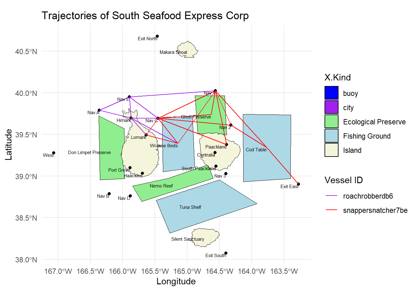
4.1 Understanding the sequence of event before South Seafood Express Corp was caught.

4.1.1 Timeline that South Seafood Express was caught - Estimated date: 2035-05-14 onward.

Steps taken:

1. Plot common vessel movement for South Seafood Express Vessels, namely “snappersnatcher7be” and “roachrobberdb6” - Reference code chunk in EDA
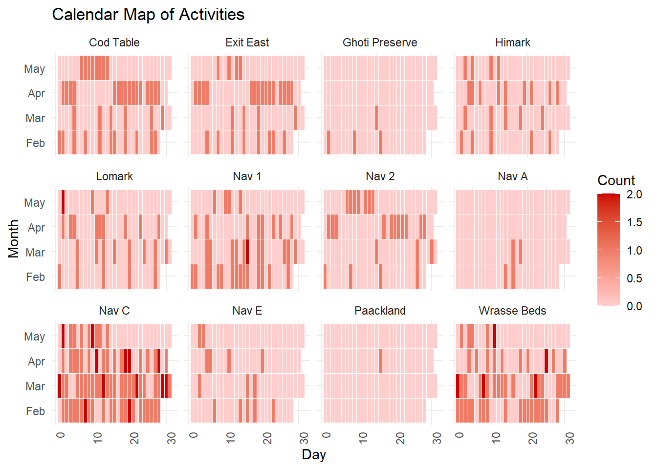
2. Plot calendar map to identify vessel pattern over time and zoom into period where South Seafood Express Vessels were still active.
3. Return data table of the last records of Transponder Ping for South Seafood Express Vessels.

Insights on South Seafood Express Corp last pings.

• 14 May 2035 for snappersnatcher7be at City of Lomark, Cod Table

• 6 May 2035 for roachrobberdb6 for City of Himark, Cod Table, Wrasse Bed

• Most vessels identified at Cod Table based on Transponder Ping, whereas for South Seafood Express Corp vessels, most activity at Nav C and Wrasse Beds

# coords <- st_coordinates(OceanusLocations)
# 
# # drop geometry columns
# OceanusLocations_df <- OceanusLocations %>%
#   st_drop_geometry()
# 
# # append x and y coordinates into df as columns
# OceanusLocations_df$XCOORD <- coords[, "X"]
# OceanusLocations_df$YCOORD <- coords[, "Y"]
# 
# # tidy df by renaming column 
# OceanusLocations_df <- OceanusLocations_df %>%
#   select(Name, X.Kind, XCOORD, YCOORD) %>%
#   rename(Loc_Type = X.Kind)
# 
# # left join to append back to vessel movement 
# 
# vessel_movement <- vessel_movement %>%
#   left_join(OceanusLocations_df,
#             by = c("area" = "Name"))
# 
# # convert vessel movement sf from point into linestring features known as vessel trajectory
# vessel_trajectory <- vessel_movement_sf %>%
#   group_by(vessel_id) %>%
#   summarize(do_union = FALSE) %>%
#   st_cast("LINESTRING")
# 
# ## include placeholder for vessel of interest and colors assigned
# 
# vessels_of_interest <- c("snappersnatcher7be", "roachrobberdb6")
# vessel_colors <- c("snappersnatcher7be" = "red", "roachrobberdb6" = "purple")
# 
# # creating route for selected vessel 
# vessel_trajectory_selected <- vessel_trajectory %>%
#   filter(vessel_id %in% vessels_of_interest)
# 
# # defining colors for X.kind
# 
# kind_colors <- c(
#   "Island" = "beige", 
#   "Fishing Ground" = "lightblue", 
#   "Ecological Preserve" = "lightgreen", 
#   "city" = "purple", 
#   "buoy" = "blue")
# 
# ggplot() +
#   geom_sf(data = oceanus_geog, aes(fill = X.Kind), color = "black") +
#   scale_fill_manual(values = kind_colors) + 
#   geom_sf(data = vessel_trajectory_selected, 
#           aes(color = vessel_id), 
#           size = 1) +
#   scale_color_manual(values = vessel_colors) + 
#   geom_text(data = OceanusLocations_df, 
#             aes(x = XCOORD, y = YCOORD, label = Name), 
#             size = 2, hjust = 1, vjust = 1) +
#   theme_minimal() +
#   labs(title = "Trajectories of South Seafood Express Corp", 
#        x = "Longitude", y = "Latitude", color = "Vessel ID")

# plotting summary of vessel movement 
vessel_movement <- vessel_movement %>%  
  mutate(year = year(start_time),
         month = month(start_time, label = TRUE),
         day = day(start_time),
         week = week(start_time),
         weekday = wday(start_time, label = TRUE, week_start = 1))

# unique(vessel_movement$area)
# focus on specific areas 

selected_area <- c("Ghoti Preserve", "Wrasse Beds", "Nemo Reef", "Don Limpet Preserve", "Tuna Shelf", "Cod Table")
selected_port <- c("Haacklee", "Lomark", "Himark", "South Paackland")
  
vessel_dist_count <- vessel_movement %>%
  group_by(area, year, month, day) %>%
  summarise(vessel_count = n_distinct(vessel_id)) %>% 
  filter(area %in% selected_area)

calendar_data <- expand.grid(year = unique(vessel_dist_count$year),
                             month = unique(vessel_dist_count$month),
                             day = 1:31, 
                             area = selected_area ) %>%
  filter(!is.na(ymd(paste(year, month, day, sep = "-"))))

# merging calendar grid with vessel count
calendar_data2 <- left_join(calendar_data, vessel_dist_count, by = c("year", "month", "day", "area"))

# sanitising by replacing NA with 0
calendar_data2$vessel_count[is.na(calendar_data2$vessel_count)] <- 0

# plotting calendar chart 
ggplot(calendar_data2, aes(x = day, y = month, fill = vessel_count)) +
  geom_tile(color = "white") +
  scale_fill_gradient(low = "#CCFFFF", high = "#006666") +
  facet_wrap(~ area ) +
  labs(title = "Calendar Map of Activities",
       x = "Day",
       y = "Month",
       fill = "Count") +
  theme_minimal() +
  theme(axis.text.x = element_text(angle = 90, hjust = 1))

# Zooming into South Seafood Express Corp activity

vessel_movement_ss <- vessel_movement %>% 
  filter(vessel_company == "SouthSeafood Express Corp") %>%
  group_by(area, year, month, day) %>%
  summarise(vessel_count = n_distinct(vessel_id))

# Exploring where SS were at - Exclude Nav areas, and Exit 
# unique(vessel_movement_ss$area)

calendar_data_ss <- expand.grid(year = unique(vessel_movement_ss$year),
                             month = unique(vessel_movement_ss$month),
                             day = 1:31, 
                             area = vessel_movement_ss$area ) %>%
  filter(!is.na(ymd(paste(year, month, day, sep = "-"))))

calendar_datass2 <- left_join(calendar_data_ss, vessel_movement_ss, by = c("year", "month", "day", "area"))

# sanitising by replacing NA with 0
calendar_datass2$vessel_count[is.na(calendar_datass2$vessel_count)] <- 0

# plotting calendar chart 
ggplot(calendar_datass2, aes(x = day, y = month, fill = vessel_count)) +
  geom_tile(color = "white") +
  scale_fill_gradient(low = "#FFCCCC", high = "#CC0000") +
  facet_wrap(~ area ) +
  labs(title = "Calendar Map of Activities",
       x = "Day",
       y = "Month",
       fill = "Count") +
  theme_minimal() +
  theme(axis.text.x = element_text(angle = 90, hjust = 1))

# return data table of last ping activity for South Seafood Express Corp

ping_activity_ss <- ping_activity %>% 
  filter(vessel_company == "SouthSeafood Express Corp") %>% 
  mutate(date = as.Date(start_time)) %>% 
  select(date, vessel_id, area ) %>%
  distinct()

datatable(ping_activity_ss, 
          options = list(pageLength = 5), 
          filter = "top")

Show 5102550100 entries

Search:

	date	vessel_id	area
	2035-02-01 2035-05-14
1	2035-03-11	roachrobberdb6	City of Lomark
2	2035-03-24	roachrobberdb6	City of Lomark
3	2035-04-04	roachrobberdb6	City of Lomark
4	2035-04-12	roachrobberdb6	City of Lomark
5	2035-04-13	roachrobberdb6	City of Lomark

Showing 1 to 5 of 353 entries

Previous12345…71Next

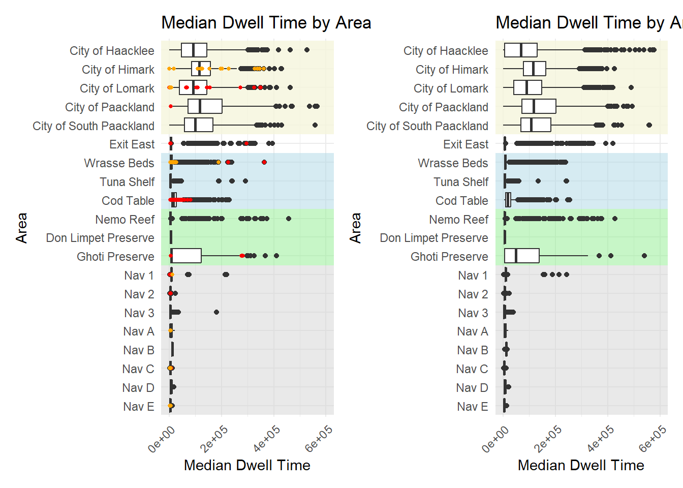
4.1.2. Looking at where South Seafood Express Corp commonly spend their time fishing at.

Steps taken:

1. Segment Transponder Ping records into 2 subset of before and after date_caught
2. Plot the median dwell time spent by South Seafood Express Vessels in comparison to other vessels
3. Contrast with the median time spent by vessels if there’s any change after date_caught.

Insights:

1. For “snappersnatcher7be” (highlighted in orange), most prominent activity in City of Himark, Wrasse Beds.
2. For “roachrobberdb6” (highlighted in red), most prominent activity in City of Lomark, and 2 instance with exceptionally long dwell time in Wrasse Beds, and majority of the time spent in Cod Table, which indicates possibility of over-fishing in these areas.
3. Also, there is a red flag for “roachrobberdb6” where it has significantly high dwell time in “Ghoti Reserve”, which is not meant for fishing.

# segment transponder ping record to before date caught and after. 
date_caught <- as.Date("2035-05-14")

fish_v_activity_bef <- fish_v_activity %>% 
mutate(start_date = as.Date(start_time)) %>%
filter(start_date <= date_caught)

fish_v_activity_aft <- fish_v_activity %>% 
mutate(start_date = as.Date(start_time)) %>%
filter(start_date > date_caught)

# assigning order to the plot
fish_v_activity_bef$area <- factor(fish_v_activity_bef$area, levels = c("Nav E", "Nav D", "Nav C" , "Nav B", "Nav A" , "Nav 3", "Nav 2", "Nav 1", "Ghoti Preserve", "Don Limpet Preserve", "Nemo Reef", "Cod Table","Tuna Shelf","Wrasse Beds","Exit East", "City of South Paackland", "City of Paackland","City of Lomark","City of Himark","City of Haacklee","City of Port Grove"))

fish_v_activity_aft$area <- factor(fish_v_activity_aft$area, levels = c("Nav E", "Nav D", "Nav C" , "Nav B", "Nav A" , "Nav 3", "Nav 2", "Nav 1", "Ghoti Preserve", "Don Limpet Preserve", "Nemo Reef", "Cod Table","Tuna Shelf","Wrasse Beds","Exit East", "City of South Paackland", "City of Paackland","City of Lomark","City of Himark","City of Haacklee","City of Port Grove"))

# plot dwell time bef and after 
fishing_dwell_bef <- ggplot(fish_v_activity_bef, aes(x = area, y = dwell)) +
  annotate("rect", ymin = -Inf, ymax = Inf, xmin = 15.5 , xmax = 20.5, alpha = 0.8, fill = "beige") +    # Ports
  annotate("rect", ymin = -Inf, ymax = Inf, xmin = 11.5, xmax = 14.5, alpha = 0.5, fill = "lightblue") +  # Fishing ground
  annotate("rect", ymin = -Inf, ymax = Inf, xmin = 8.5, xmax = 11.5, fill = "lightgreen", alpha = 0.5) +  # Ecological preserve
  annotate("rect", ymin = -Inf, ymax = Inf, xmin = 0.5, xmax = 8.5, alpha = 0.5, fill = "lightgrey") +
  geom_boxplot() +
  geom_point(data = subset(fish_v_activity_bef, vessel_id == "snappersnatcher7be"),
             aes(x = area, y = dwell), color = "red", size = 1) +
  geom_point(data = subset(fish_v_activity_bef, vessel_id == "roachrobberdb6"),
             aes(x = area, y = dwell), color = "orange", size = 1) +
  theme_minimal() +
  labs(title = "Median Dwell Time by Area", 
       x = "Area", 
       y = "Median Dwell Time") +
  theme(axis.text.x = element_text(angle = 45, hjust = 1)) + 
  scale_y_continuous(limits = c(0, 600000)) + # limit dwell 
  coord_flip()

fishing_dwell_aft <- ggplot(fish_v_activity_aft, aes(x = area, y = dwell)) +
  annotate("rect", ymin = -Inf, ymax = Inf, xmin = 15.5 , xmax = 20.5, alpha = 0.8, fill = "beige") +    # Ports
  annotate("rect", ymin = -Inf, ymax = Inf, xmin = 11.5, xmax = 14.5, alpha = 0.5, fill = "lightblue") +  # Fishing ground
  annotate("rect", ymin = -Inf, ymax = Inf, xmin = 8.5, xmax = 11.5, fill = "lightgreen", alpha = 0.5) +  # Ecological preserve
  annotate("rect", ymin = -Inf, ymax = Inf, xmin = 0.5, xmax = 8.5, alpha = 0.5, fill = "lightgrey") +
  geom_boxplot() +
  theme_minimal() +
  labs(title = "Median Dwell Time by Area", 
       x = "Area", 
       y = "Median Dwell Time") +
  theme(axis.text.x = element_text(angle = 45, hjust = 1)) + 
  scale_y_continuous(limits = c(0, 600000)) + # limit dwell 
  coord_flip()

fishing_dwell_bef | fishing_dwell_aft

4.2 Visualizing changes to other vessels & cargo after South Seafood Express was caught.

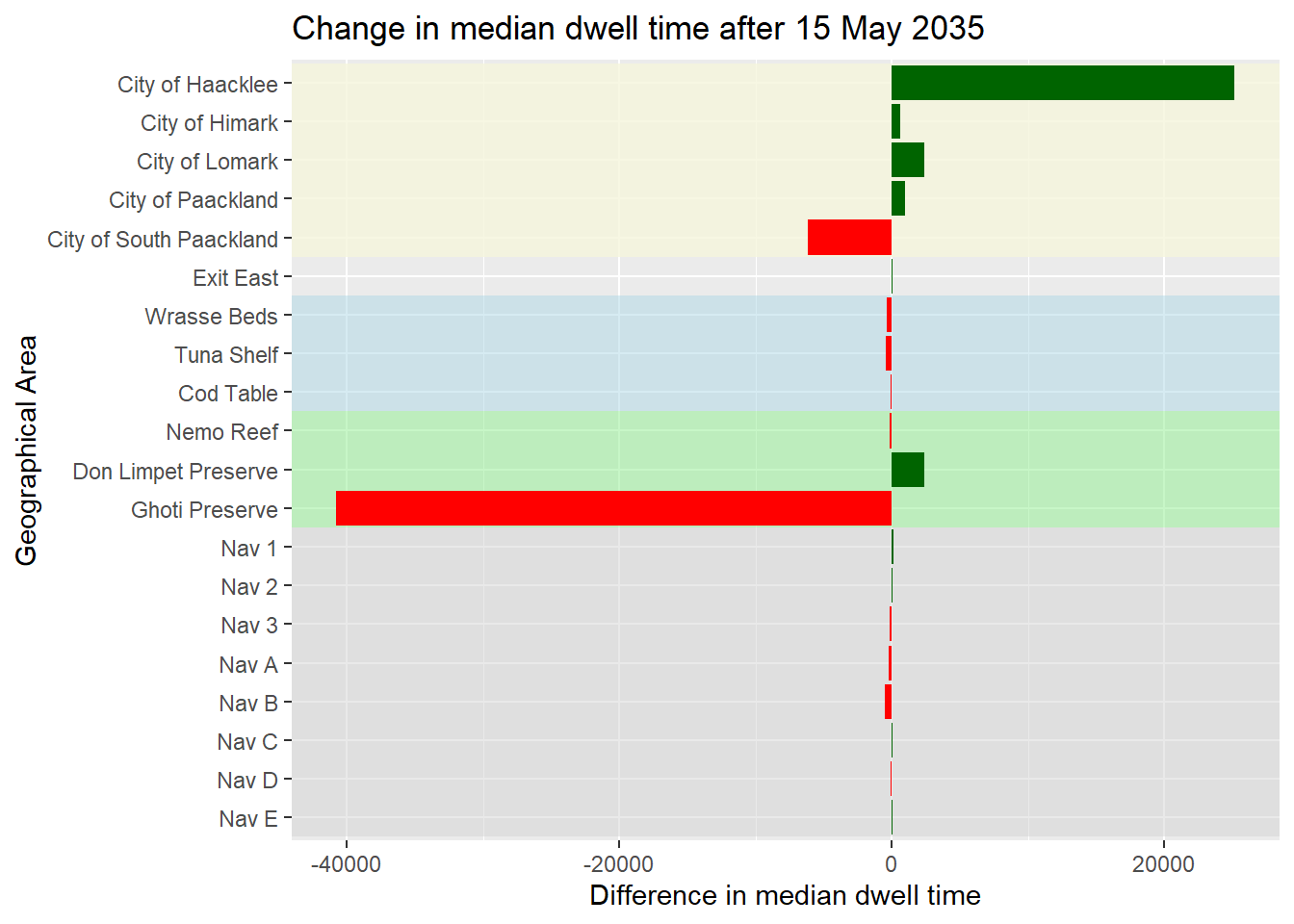
4.2.1 How median dwell time have changed

Insights:

1. Drastic decrease in median dwell time for “Ghoti Reserve” after South Seafood Express Corp has been caught.
2. Likely that vessels either stop their illegal fishing or they routed over to “Don Limpet Reserve” where we see a slight increase in the median dwell time.
3. Substantial increase in median dwell time at City of Paackland, pointing to possible vessels seeking shelter, till the aftermath and scrutiny on South Seafood Express Corp illegal activities investigation has ceased.

# comparing median time spent at each area before and after

fish_v_activity_bef_sum <- fish_v_activity_bef %>%
  group_by(area) %>%
  summarise(median_dwell = median(dwell, na.rm = TRUE))

fish_v_activity_aft_sum <- fish_v_activity_aft %>%
  group_by(area) %>%
  summarise(median_dwell = median(dwell, na.rm = TRUE))

fish_v_bef_aft <- left_join(fish_v_activity_bef_sum, fish_v_activity_aft_sum, by = c("area" = "area"))
fish_v_bef_aft <- fish_v_bef_aft %>% 
  rename(median_dwell_bef = median_dwell.x, median_dwell_aft = median_dwell.y) %>%
  mutate(diff_bef_aft = median_dwell_bef - median_dwell_aft) %>% arrange(diff_bef_aft)

# reorder 
fish_v_bef_aft$area <- factor(fish_v_bef_aft$area, levels = c("Nav E", "Nav D", "Nav C" , "Nav B", "Nav A" , "Nav 3", "Nav 2", "Nav 1", "Ghoti Preserve", "Don Limpet Preserve", "Nemo Reef", "Cod Table","Tuna Shelf","Wrasse Beds","Exit East", "City of South Paackland", "City of Paackland","City of Lomark","City of Himark","City of Haacklee","City of Port Grove"))

ggplot(fish_v_bef_aft, 
       aes(x= area, y = diff_bef_aft, fill = diff_bef_aft >0)) + 
  annotate("rect", ymin = -Inf, ymax = Inf, xmin = 15.5 , xmax = 20.5, alpha = 0.8, fill = "beige") +    # Ports
  annotate("rect", ymin = -Inf, ymax = Inf, xmin = 11.5, xmax = 14.5, alpha = 0.5, fill = "lightblue") +  # Fishing ground
  annotate("rect", ymin = -Inf, ymax = Inf, xmin = 8.5, xmax = 11.5, fill = "lightgreen", alpha = 0.5) +  # Ecological preserve
  annotate("rect", ymin = -Inf, ymax = Inf, xmin = 0.5, xmax = 8.5, alpha = 0.5, fill = "lightgrey") +
  geom_bar(stat = "identity") +
  scale_fill_manual(values = c("TRUE" = "darkgreen", "FALSE" = "red"), guide = FALSE) + 
  labs(title = "Change in median dwell time after 15 May 2035", 
       x = "Geographical Area", 
       y = "Difference in median dwell time") + 
  coord_flip()

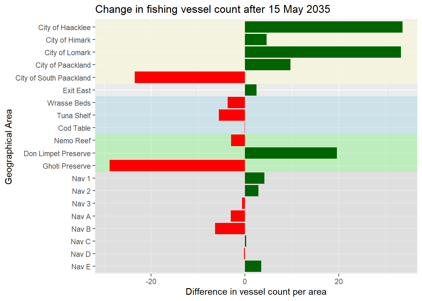
4.2.2 How count of vessels in each area has changed

Insights:

1. General decrease in vessel count at the various ports. This might point to some vessels which are idle after South Seafood Express Corp was caught.
2. Possibly change in the location where vessels were identified from “Wrasse Beds” and “Cod Table” to “Tuna Shelf”. This might be due to seasonality of fish catch that requires further analysis on the expected cargo for Oceanus over the years.
3. Decrease in vessel count in “Nav C” nearer to Ghoti Reserve, and increase in “Nav D” nearer to Nemo Reefs, which potentially point to vessels shifting away from sensitive area of “Ghoti Reserve” under tight scrutiny to continue their illegal fishing activities in “Nemo Reefs”

fish_v_activity_bef_count <- fish_v_activity_bef %>%
  group_by(start_date, area) %>%
  summarize(fish_dist_count_bef = n_distinct(vessel_id)) %>% 
  group_by(area) %>% 
  summarize (fish_dist_total_bef = sum(fish_dist_count_bef))

# adjustment to moderate count by week 

days_bef <- difftime(date_caught, min(fish_v_activity_bef$start_date),  units = "days") #102 days --> /7 for weeks
days_aft <- difftime(max(fish_v_activity_aft$start_date), date_caught, units = "days") #199 days 

fish_v_activity_aft_count <- fish_v_activity_aft %>%
  group_by(start_date, area) %>%
  summarize(fish_dist_count_aft = n_distinct(vessel_id)) %>% 
  group_by(area) %>% 
  summarize (fish_dist_total_aft = sum(fish_dist_count_aft)) 

fish_v_count_bef_aft <- left_join(fish_v_activity_bef_count, fish_v_activity_aft_count, by = c("area" = "area"))
fish_v_count_bef_aft <- fish_v_count_bef_aft %>% 
  mutate(fish_dist_total_bef_weeks = (fish_dist_total_bef / as.numeric(days_bef))*7, 
          fish_dist_total_aft_weeks = (fish_dist_total_aft/ as.numeric(days_aft))*7) %>% 
  mutate(diff_count_bef_aft = fish_dist_total_bef_weeks - fish_dist_total_aft_weeks) %>% 
  arrange(diff_count_bef_aft)

# reorder 
fish_v_count_bef_aft$area <- factor(fish_v_bef_aft$area, levels = c("Nav E", "Nav D", "Nav C" , "Nav B", "Nav A" , "Nav 3", "Nav 2", "Nav 1", "Ghoti Preserve", "Don Limpet Preserve", "Nemo Reef", "Cod Table","Tuna Shelf","Wrasse Beds","Exit East", "City of South Paackland", "City of Paackland","City of Lomark","City of Himark","City of Haacklee","City of Port Grove"))

# plot

ggplot(fish_v_count_bef_aft, 
       aes(x= area, y = diff_count_bef_aft, fill = diff_count_bef_aft >0)) +
  annotate("rect", ymin = -Inf, ymax = Inf, xmin = 15.5 , xmax = 20.5, alpha = 0.8, fill = "beige") +    # Ports
  annotate("rect", ymin = -Inf, ymax = Inf, xmin = 11.5, xmax = 14.5, alpha = 0.5, fill = "lightblue") +  # Fishing ground
  annotate("rect", ymin = -Inf, ymax = Inf, xmin = 8.5, xmax = 11.5, fill = "lightgreen", alpha = 0.5) +  # Ecological preserve
  annotate("rect", ymin = -Inf, ymax = Inf, xmin = 0.5, xmax = 8.5, alpha = 0.5, fill = "lightgrey") +
  geom_bar(stat = "identity") + 
  scale_fill_manual(values = c("TRUE" = "darkgreen", "FALSE" = "red"), guide = FALSE) + 
  labs(title = "Change in fishing vessel count after 15 May 2035", 
       x = "Geographical Area", 
       y = "Difference in vessel count per area") + 
  coord_flip()

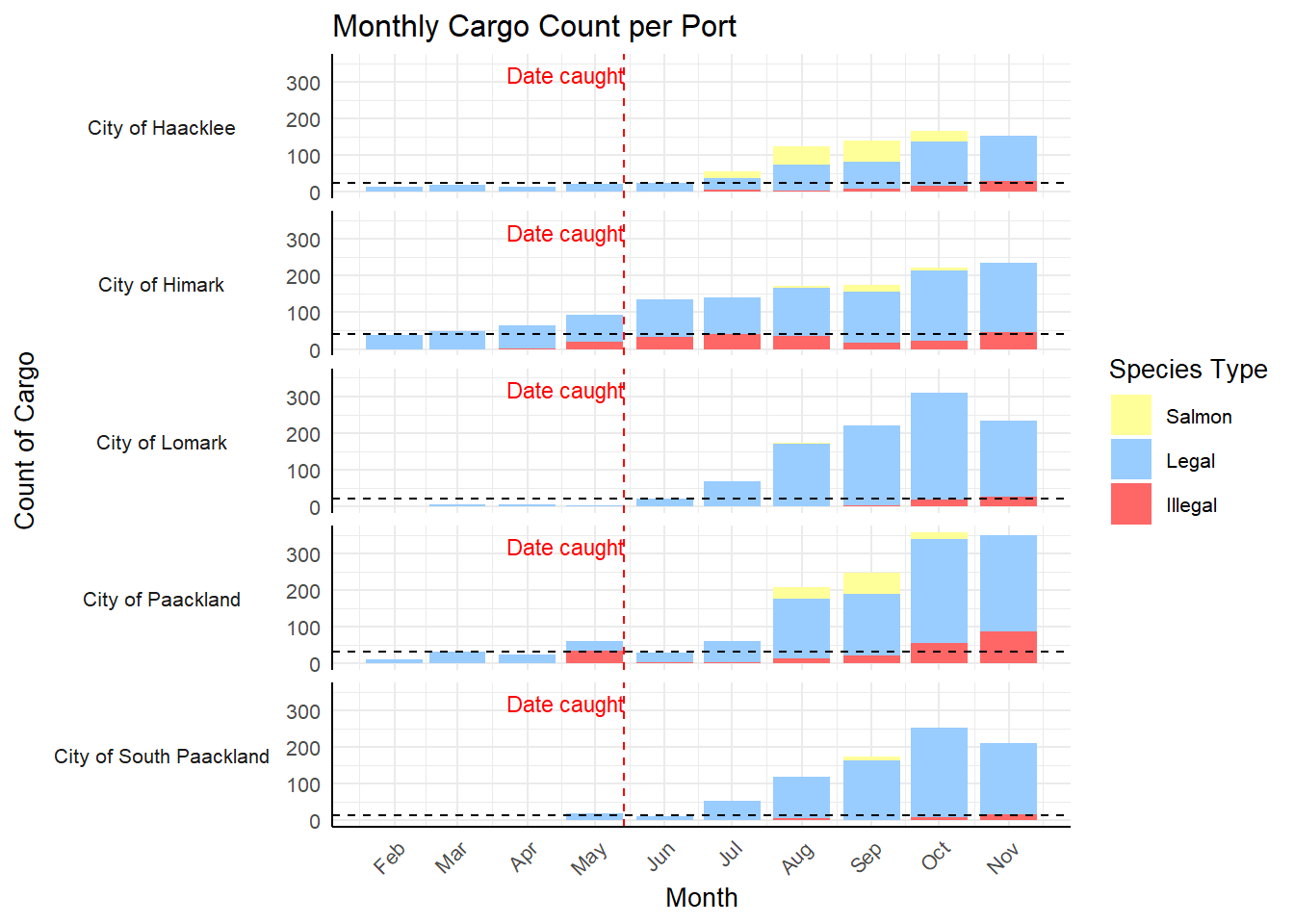
4.2.3 How cargo count have changed over time.

Insights:

1. General increase in cargo count across the month of May till November and this is likely due to the seasonality of the fish stock in the ocean.
2. However, notable changes include City of Himark where there is a drop in cargo count of illegal fish species from July, May till September. On the contrary, the illegal cargo count for City of Paackland and City of Lomark has increased from Auguest till November where it peaked.
3. City of Haacklee and Paackland has a substantial proportion of cargo belonging to “Salmon” fish species, and this may be due to the relative proximity to the south fringes of Oceanus islands.

# including date that south seafood was caught
date_caught <- as.Date("2035-05-14")


# coloring by illegal fish species 
cargo_color <- c("Legal" = "#99CCFF", "Salmon" = "#FFFF99", "Illegal" = "#FF6666")

illegal_species = c("piscesfoetidaae7", "piscisosseusb6d", "piscessatisb87")
legal_species =  c("gadusnspecificatae4ba", "piscissapidum9b7", "habeaspisces4eb", "piscesfrigus900", "labridaenrefert9be", "thunnininveradb7")
salmon = c("oncorhynchusrosea790")

cargo_summary <- tx_qty %>%
  mutate(month = floor_date(as.Date(tx_date), "month"), 
         species_type = case_when(
           fish_species %in% illegal_species ~ "Illegal", 
           fish_species %in% legal_species ~ "Legal", 
           fish_species %in% salmon ~ "Salmon"
         )) %>%
  group_by(dest, month, species_type) %>%
  summarize(cargo_count = n()) 

#refactoring to put illegal species at bottom
cargo_summary$species_type <- factor(cargo_summary$species_type, levels = c("Salmon", "Legal", "Illegal"))

# calculating median and total cargo count for annotation

median_counts <- cargo_summary %>%
  group_by(dest) %>%
  summarize(median_count = median(cargo_count))

# Plot the stacked bar graph with reference lines and text labels
ggplot(cargo_summary, aes(x = month, y = cargo_count, fill = species_type)) +
  geom_bar(stat = "identity") +
  scale_fill_manual(values = cargo_color) +  # Set the custom colors
  geom_hline(data = median_counts, aes(yintercept = median_count), linetype = "dashed", color = "black") +
  geom_vline(xintercept = as.numeric(date_caught), linetype = "dashed", color = "red") +
  scale_x_date(date_breaks = "1 month", date_labels = "%b") + 
  labs(title = "Monthly Cargo Count per Port",
       x = "Month",
       y = "Count of Cargo",
       fill = "Species Type") +
  facet_grid(dest ~ ., switch = "y") +
  theme_minimal(base_size = 10) +
  theme(axis.text.x = element_text(angle = 45, hjust = 1),
        axis.line = element_line(color = "black"),
        strip.background = element_blank(),
        strip.placement = "outside",
        strip.text.y.left = element_text(angle = 0)) + 
   annotate("text", x = date_caught, y = 320, label = "Date caught", color = "red", hjust = 1, size = 3)

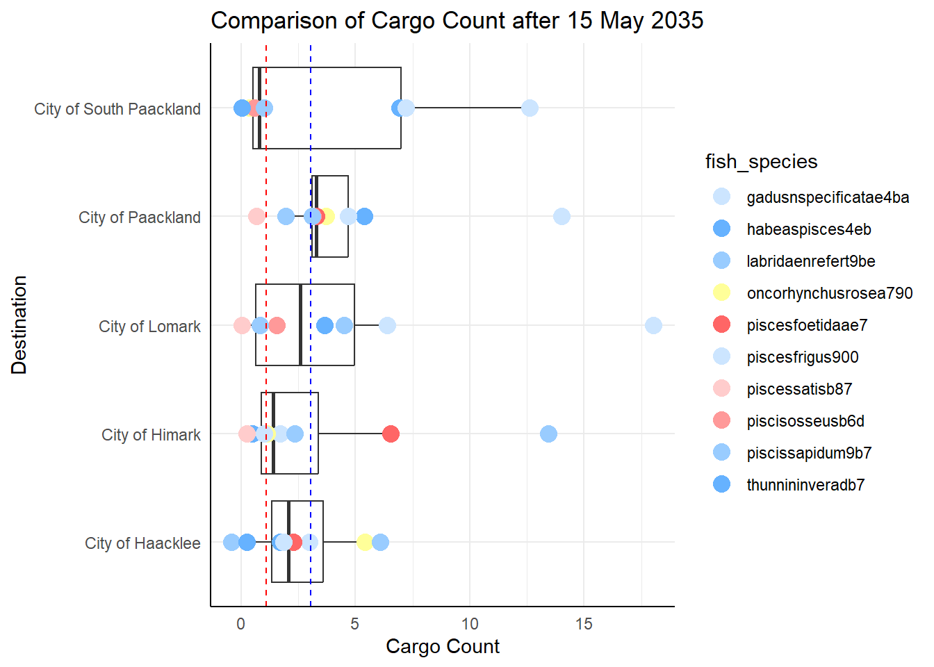
4.2.4 How cargo quantity has changed

Insights:

1. In general the quantity of fish species caught have increased. This is aligned with the seasonal trend where there is more catches in the later part of the year with warmer waters and post fish breeding.
2. However, exceptional points include unusually huge increase in illegal fish species of “piscesfoetidaae7” reported at “City of Himark” which may point to illegal fishing at “Don Limpet Preserve”.
3. There is also exception increase in “Salmon” quantity reported at City of Haacklee, pointing to possible fishing in unregulated waters.
4. Comparing the rate of increase in fish quantity caught, while illegal fish quantity increase is on average lower than legal fish quantity increase, there is still notable increase in cargo unloaded at “City of Paackland, City of Himark and City of Haacklee”.

tx_qty_bef <- tx_qty1 %>% filter(tx_date <= date_caught)
tx_qty_aft <- tx_qty1 %>% filter(tx_date > date_caught)

# Calculate median quantity of fish per port 
tx_qty_bef_sum <- tx_qty_bef %>% 
  group_by(dest, fish_species) %>%
  summarize(qty_tons_bef_sum = sum(qty_tons), cargo_bef_count = n())

tx_qty_aft_sum <- tx_qty_aft %>%
  group_by(dest, fish_species) %>%
  summarize(qty_tons_aft_sum = sum(qty_tons), cargo_aft_count = n())

tx_qty_bef_aft <- left_join(tx_qty_aft_sum, tx_qty_bef_sum, by = c("dest" = "dest", "fish_species" = "fish_species"))

colnames(tx_qty_bef_aft)

[1] "dest"             "fish_species"     "qty_tons_aft_sum" "cargo_aft_count" 
[5] "qty_tons_bef_sum" "cargo_bef_count" 

# adjustment to per week
tx_qty_bef_aft <- tx_qty_bef_aft %>% 
  mutate(qty_tons_aft_sum_week = (qty_tons_aft_sum / as.numeric(days_aft))*7,
        cargo_aft_count_week = (cargo_aft_count / as.numeric(days_aft))*7, 
qty_tons_bef_sum_week = (qty_tons_bef_sum / as.numeric(days_bef))*7,
cargo_bef_count_week = (cargo_bef_count / as.numeric(days_bef))*7)

tx_qty_bef_aft <- tx_qty_bef_aft %>%
  mutate(across(everything(), ~ replace_na(.x, 0)), 
         qty_tons_bef_aft_week = qty_tons_aft_sum_week - qty_tons_bef_sum_week, 
         cargo_count_bef_aft_week = cargo_aft_count_week - cargo_bef_count_week)

# draw hline for legal and illegal fishes
tx_qty_bef_aft_legal <- tx_qty_bef_aft %>% 
  filter(fish_species %in% 
           c("gadusnspecificatae4ba", "piscissapidum9b7", "habeaspisces4eb", "piscesfrigus900", "labridaenrefert9be", "thunnininveradb7") )

median_count_legal <- median(tx_qty_bef_aft_legal$cargo_count_bef_aft_week, na.rm = TRUE)
median_qty_legal <- median(tx_qty_bef_aft_legal$qty_tons_bef_aft_week, na.rm = TRUE)

tx_qty_bef_aft_illegal <- tx_qty_bef_aft %>% 
  filter(fish_species %in% c("piscesfoetidaae7", "piscisosseusb6d", "piscessatisb87") )
median_count_illegal <- median(tx_qty_bef_aft_illegal$cargo_count_bef_aft_week, na.rm = TRUE)
median_qty_illegal <- median(tx_qty_bef_aft_illegal$qty_tons_bef_aft_week, na.rm = TRUE)

# assign color by fish species
fish_species_color <- c("piscesfoetidaae7" = "#FF6666", 
                        "piscisosseusb6d" = "#FF9999", 
                        "piscessatisb87" = "#FFCCCC", 
                        "gadusnspecificatae4ba" = "#CCE5FF", 
                        "piscissapidum9b7" = "#99CCFF", 
                        "habeaspisces4eb" = "#66B2ff", 
                        "piscesfrigus900" = "#CCE5FF", 
                        "oncorhynchusrosea790" = "#FFFF99", 
                        "labridaenrefert9be" = "#99CCFF", 
                        "thunnininveradb7" = "#66b2ff"
                        )

# plot
tx_count_bef_aft <- ggplot(tx_qty_bef_aft, 
                           aes(x = dest, y = cargo_count_bef_aft_week)) +
  theme_minimal() + 
  theme(axis.line = element_line(color = "black")) +
  geom_boxplot() + 
  geom_point(aes(color = fish_species), size = 4) + 
  geom_hline(aes(yintercept = median_count_legal), 
             color = "blue", linetype = "dashed") + 
  geom_hline(aes(yintercept = median_count_illegal), color = "red", linetype = "dashed")+ 
  scale_color_manual(values = fish_species_color) + 
  coord_flip() + 
  labs(title = "Comparison of Cargo Count after 15 May 2035", 
        x = "Destination", y = "Cargo Count") 


plot_tx_qty_bef_aft <- ggplot(tx_qty_bef_aft, 
                              aes(x= dest, y = qty_tons_bef_aft_week)) +
  theme_minimal() + 
  theme(axis.line = element_line(color = "black")) +
  geom_boxplot() + 
  geom_point(aes(color = fish_species), size = 4) + 
  geom_hline(aes(yintercept = median_qty_legal), 
             color = "blue", linetype = "dashed") + 
  geom_hline(aes(yintercept = median_qty_illegal), color = "red", linetype = "dashed")+ 
  scale_color_manual(values = fish_species_color) +  
  coord_flip() + 
  labs(title = "Comparison of Cargo Quantity after 15 May 2035", 
       x = "Destination", y = "Cargo Quantity in tons")

tx_count_bef_aft

plot_tx_qty_bef_aft

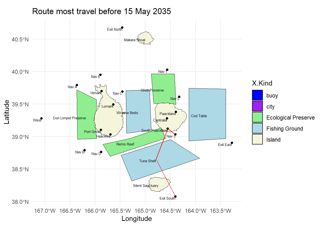
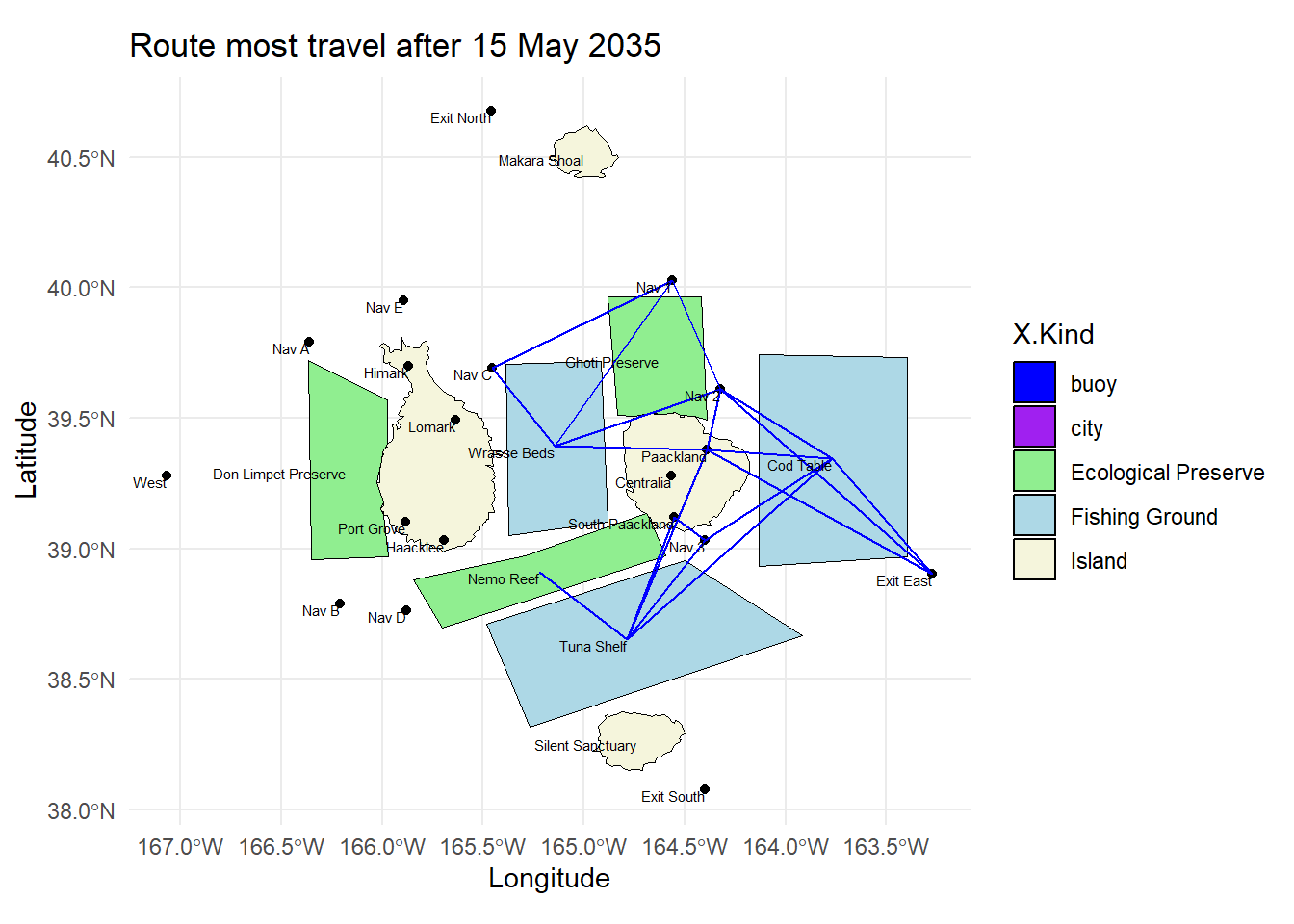
4.2.5. How travel routes have changed

Insights:

1. Shift of most popular route before and after 15 May 2023, this is likely due to the availability of fishes within the fishing region during the fishing season, unlike previously where the ships have to go outskirts to fish.
2. Exponential increase in vessels activity after 15 May 2023, and this can be seen by the summary table below.

Most Popular Route before 15 May 2023	Most Popular Route After 15 May 2023
Location: City of Himark, Nav 3, Exit East, Cod Table, Exit North, Exit South, West, Nav 2, City of Paackland, Tuna Shelf, etc. Vessel Count: 85 Unique vessels: 1 (seawaysynergybaf)	Location: City of Paackland, Nav 2, Cod Table, Exit East Vessel Count: 375 Unique vessels: 15 (haddockhunter1a7 eelenthusiast8c6 sardineseeker62e marinersmate8ee baitedbreath538 seabreamseekerd8b speckledtroutsaboteur509 americaneelenthusiastcfa tarpontaker6cd wahoowarriord42 longfintunalooterf32 marlinmaster8ab wahoowrangler016 dolphindasher004 goldentroutgrabber7f6

Further insights to be derived by:

1. Segmenting the route behaviour into more granular subset for comparison. E.g., The 3 subsets identified in EDA for unusually large fishing vessels, foreign unusually small cargo vessels, and foreign exceptionally large cargo vessels.
2. Comparison to the cargo deposited by each dominant route to identify any under-reporting of catch by certain vessels and companies.

route_vessel_summary_full <- nearest_tx_date %>%
  group_by(route_list) %>%
  summarize(vessel_count = n_distinct(vessel_id))

# Extract unique locations within a path

route_vessel_summary_path_only <- nearest_tx_date %>% 
  mutate(unique_areas = str_split(route_list, ", ") %>% 
                       map(~ unique(.x) %>% paste(collapse = ", ")))

# count the number of vessel occurence and unique vessel count 

route_summary_count <- route_vessel_summary_path_only %>% 
  group_by(unique_areas) %>%
  summarize(vessel_count = n(), 
            unique_vessel_count = n_distinct(vessel_id)) %>%
  arrange(- vessel_count)

# before and after # 127 distinct routes
route_vessel_bef <- route_vessel_summary_path_only %>% 
  filter(tx_date <= date_caught) %>% 
  group_by(unique_areas) %>%
  summarise(
    vessel_count = n(), 
    unique_vessel_count = n_distinct(vessel_id),
    unique_vessels = toString(unique(vessel_id))
  ) 

route_vessel_bef <- route_vessel_bef %>% arrange(desc(vessel_count))

datatable(route_vessel_bef, options = list(pageLength = 3))

Show 3102550100 entries

Search:

	unique_areas	vessel_count	unique_vessel_count	unique_vessels
1	City of Himark, Nav 3, Exit East, Cod Table, NA, Nav 1	85	1	seawaysynergybaf
2	City of Himark, Nav 3, Cod Table	62	1	aquatransit6bc
3	City of Paackland, Nav 2, Cod Table, Exit East	17	3	bonefishbaiter565, dolphindasher004, bassbaiterb9f

Showing 1 to 3 of 127 entries

Previous12345…43Next

# after - # 307 routes 
route_vessel_aft <- route_vessel_summary_path_only %>% 
  filter(tx_date > date_caught) %>% 
  group_by(unique_areas) %>%
  summarise(
    vessel_count = n(), 
    unique_vessel_count = n_distinct(vessel_id),
    unique_vessels = toString(unique(vessel_id))
  )

route_vessel_aft <- route_vessel_aft %>% arrange(desc(vessel_count))

datatable(route_vessel_aft, options = list(pageLength = 3))

Show 3102550100 entries

Search:

	unique_areas	vessel_count	unique_vessel_count	unique_vessels
1	City of Paackland, Nav 2, Cod Table, Exit East	375	15	haddockhunter1a7, eelenthusiast8c6, sardineseeker62e, marinersmate8ee, baitedbreath538, seabreamseekerd8b, speckledtroutsaboteur509, americaneelenthusiastcfa, tarpontaker6cd, wahoowarriord42, longfintunalooterf32, marlinmaster8ab, wahoowrangler016, dolphindasher004, goldentroutgrabber7f6
2	City of Himark, City of South Paackland, Exit East, Nav 3, Nav 1, Cod Table	373	1	cargocentric4d0
3	City of Lomark, Nav 2, Exit East, Cod Table, Nav 1, Nav C, Wrasse Beds	272	3	gurnardgrabberd9a, trawlertriumph31f, oceanoracle1d0

Showing 1 to 3 of 307 entries

Previous12345…103Next

# plot most popular route before South Seafood is caught

max_vessel_count_row <- route_vessel_bef %>% 
  filter(vessel_count == max(vessel_count))

# Extract the unique vessels from that row
vessels_of_interest_bef <- strsplit(max_vessel_count_row$unique_vessels, ", ")[[1]]

# creating route for selected vessel 
vessel_trajectory_selected <- vessel_trajectory %>%
  filter(vessel_id %in% vessels_of_interest_bef)

# defining colors for X.kind

ggplot() +
  geom_sf(data = oceanus_geog, aes(fill = X.Kind), color = "black") +
  scale_fill_manual(values = kind_colors) + 
  geom_sf(data = vessel_trajectory_selected, 
          color = "red", 
          size = 3) + 
  geom_text(data = OceanusLocations_df, 
            aes(x = XCOORD, y = YCOORD, label = Name), 
            size = 2, hjust = 1, vjust = 1) +
  theme_minimal() +
  labs(title = "Route most travel before 15 May 2035", 
       x = "Longitude", y = "Latitude", color = "Vessel ID")

# plot most popular route after South Seafood is caught
  
max_vessel_count_row <- route_vessel_aft %>% 
  filter(vessel_count == max(vessel_count))

# Extract the unique vessels from that row
vessels_of_interest_aft <- strsplit(max_vessel_count_row$unique_vessels, ", ")[[1]]

# creating route for selected vessel 
vessel_trajectory_selected <- vessel_trajectory %>%
  filter(vessel_id %in% vessels_of_interest_aft)

# defining colors for X.kind

ggplot() +
  geom_sf(data = oceanus_geog, aes(fill = X.Kind), color = "black") +
  scale_fill_manual(values = kind_colors) + 
  geom_sf(data = vessel_trajectory_selected, 
          color = "blue",  # Set the color directly
          size = 3) + 
  geom_text(data = OceanusLocations_df, 
            aes(x = XCOORD, y = YCOORD, label = Name), 
            size = 2, hjust = 1, vjust = 1) +
  theme_minimal() +
  labs(title = "Route most travel after 15 May 2035", 
       x = "Longitude", y = "Latitude", color = "Vessel ID")