Take-home Exercise 3 - Time Series

Author

Seng Jing Yi

Published

June 18, 2024

Modified

June 21, 2024

Testing out time series analysis based on mapped records

Importing packages

Code

pacman::p_load(jsonlite, tidyverse, tidyr, 
               knitr, lubridate, dplyr, 
               igraph, ggraph, ggdist, ggplot2, 
               SmartEDA, sf, tidygraph, reshape2, readr,
               DT, patchwork,plotly)

Importing data

Code

tx_qty <- read_csv("data/tx_qty.csv")
ping_activity <- read_csv("data/ping_activity.csv")
E_Hbrpt_v <- read_csv("data/hbrpt.csv")
N_vessel <- read_csv("data/N_vessel.csv")
location_legend <- read_csv("data/location_legend.csv")
NL_City <- read_csv("data/NL_City.csv")
vessel_movement <- read_rds("data/rds/vessel_movement_data.rds")
nearest_tx_date <- read_csv("data/mapped_records.csv")

Importing geographical data

Code

OceanusGeography = st_read("data/Oceanus Geography.geojson") %>%
  st_transform(crs = 4326)

Reading layer `Oceanus Geography' from data source 
  `C:\sengjingyi\ISSS608\Take-home_Ex\Take-home_Ex03\data\Oceanus Geography.geojson' 
  using driver `GeoJSON'
Simple feature collection with 29 features and 7 fields
Geometry type: GEOMETRY
Dimension:     XY
Bounding box:  xmin: -167.0654 ymin: 38.07452 xmax: -163.2723 ymax: 40.67775
Geodetic CRS:  WGS 84

Code

OceanusLocations <- st_read(dsn = "data/shp",
  layer = "Oceanus Geography")

Reading layer `Oceanus Geography' from data source 
  `C:\sengjingyi\ISSS608\Take-home_Ex\Take-home_Ex03\data\shp' 
  using driver `ESRI Shapefile'
Simple feature collection with 27 features and 7 fields
Geometry type: POINT
Dimension:     XY
Bounding box:  xmin: -167.0654 ymin: 38.07452 xmax: -163.2723 ymax: 40.67775
Geodetic CRS:  WGS 84

Code

coords <- st_coordinates(OceanusLocations)

OceanusLocations_df <- OceanusLocations %>%
  st_drop_geometry()

OceanusLocations_df$XCOORD <- coords[, "X"]
OceanusLocations_df$YCOORD <- coords[, "Y"]

OceanusLocations_df <- OceanusLocations_df %>%
  select(Name, X.Kind, XCOORD, YCOORD) %>%
  rename(Loc_Type = X.Kind)

ggplot() +
  geom_sf(data = OceanusGeography) +
  theme_minimal() +
  labs(title = "Map of Oceanus", 
  x = "Longitude", y = "Latitude", color = "ID")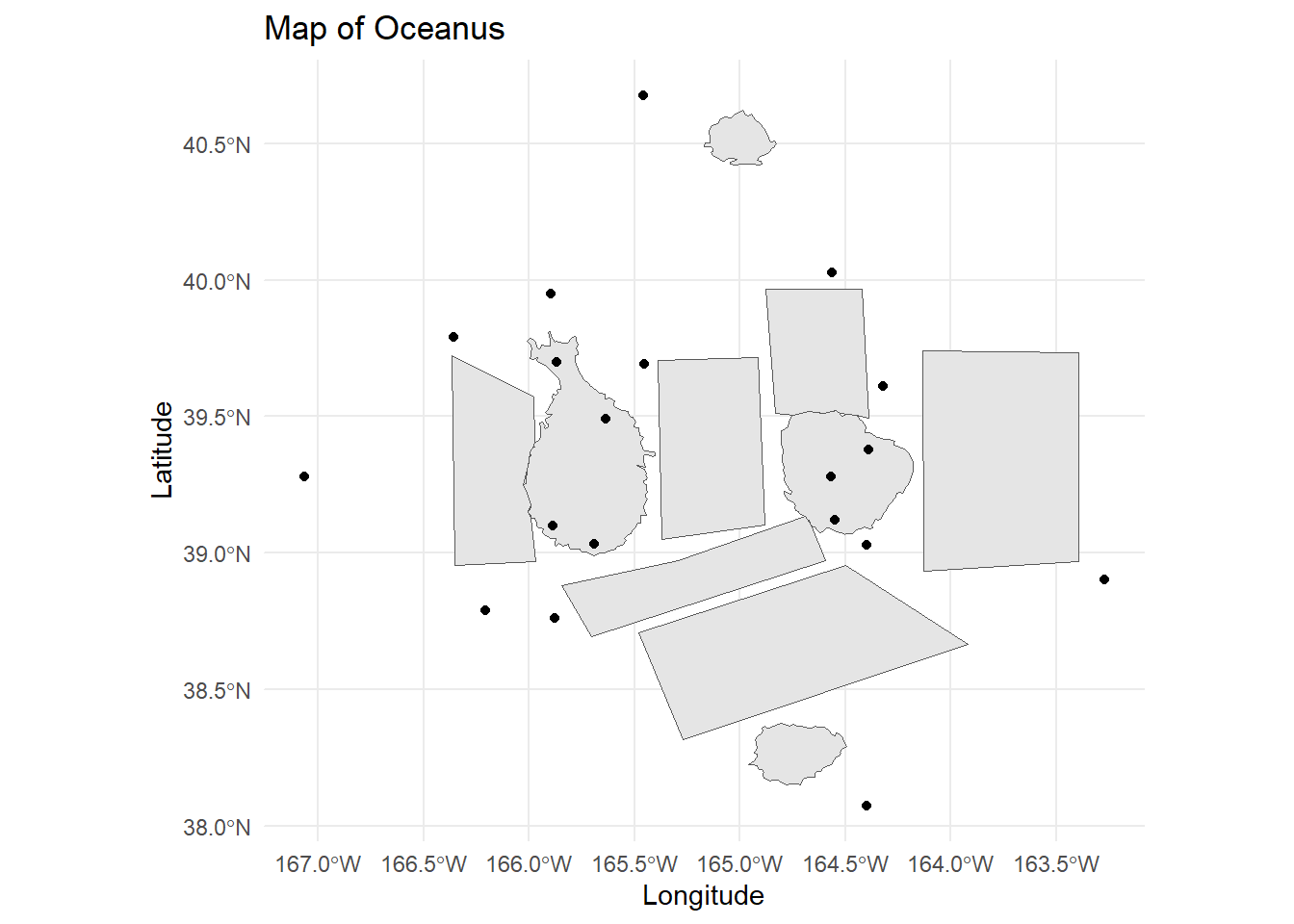

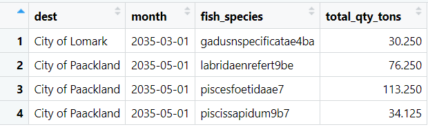
Merging the vessel details back with the mapped records in the dataframe nearest_tx_date

Code

mapped_records <- nearest_tx_date %>% 
  left_join(N_vessel %>% 
              select(vessel_id, vessel_name, flag_country, 
                     vessel_company, tonnage, length_overall, vessel_type), 
                            by = c("vessel_id" = "vessel_id"))

Exploring potentially suspicious records where matching algorithm matched to “non-fishing” vessels.

Type: Cargo_vessels
44 unique vessel_id returned for total 1898 unique cargo_ids

Code

non_fishing_match <- mapped_records %>% filter(vessel_type != "Fishing")

non_fishing_match_vessel_id <- unique(non_fishing_match$vessel_id)
non_fishing_match_cargo_count <- unique(non_fishing_match$cargo_id)

non_fishing_match_country <- non_fishing_match %>% 
  group_by(flag_country, vessel_id, fish_species) %>% 
  summarise(cargo_count = n_distinct(cargo_id))

flag_country_order <- non_fishing_match_country %>%
  group_by(flag_country) %>%
  summarise(total_cargo_count = sum(cargo_count)) %>%
  arrange(total_cargo_count) %>%
  pull(flag_country)

# Reorder flag_country based on the total cargo count
non_fishing_match_country$flag_country <- factor(non_fishing_match_country$flag_country, levels = flag_country_order)

# manually assigning fish species color
species_colors <- c(
  "gadusnspecificatae4ba" = "#FF6347",  # Illegal
  "habeaspisces4eb" = "#99CCFF",        # Legal
  "labridaenrefert9be" = "#99CCFF",     # Legal
  "piscesfoetidaae7" = "#FF6666",       # Illegal
  "piscesfrigus900" = "#99CCFF",        # Legal
  "piscessatisb87" = "#FF6666",         # Illegal
  "piscisosseusb6d" = "#FF6666",        # Illegal
  "piscissapidum9b7" = "#99CCFF",       # Legal
  "thunnininveradb7" = "#99CCFF"        # Legal
)

# Create the plot
non_fishing_match_country_plot <- ggplot(non_fishing_match_country, aes(x = flag_country, y = cargo_count, fill = fish_species)) +
  geom_bar(stat = "identity", position = "dodge") +
  labs(x = "Flag Country", y = "Cargo Count", title = "Cargo Count by Flag Country, and Fish Species", fill = "Fish Species") +
  scale_fill_manual(values = species_colors) + 
  theme(axis.text.x = element_text(angle = 45, hjust = 1), 
        legend.text = element_text(angle = 45, hjust = 1)) +
  theme_minimal() +
  facet_wrap(~ fish_species) 
  coord_flip()

<ggproto object: Class CoordFlip, CoordCartesian, Coord, gg>
    aspect: function
    backtransform_range: function
    clip: on
    default: FALSE
    distance: function
    expand: TRUE
    is_free: function
    is_linear: function
    labels: function
    limits: list
    modify_scales: function
    range: function
    render_axis_h: function
    render_axis_v: function
    render_bg: function
    render_fg: function
    setup_data: function
    setup_layout: function
    setup_panel_guides: function
    setup_panel_params: function
    setup_params: function
    train_panel_guides: function
    transform: function
    super:  <ggproto object: Class CoordFlip, CoordCartesian, Coord, gg>

Code

non_fishing_match_country_plot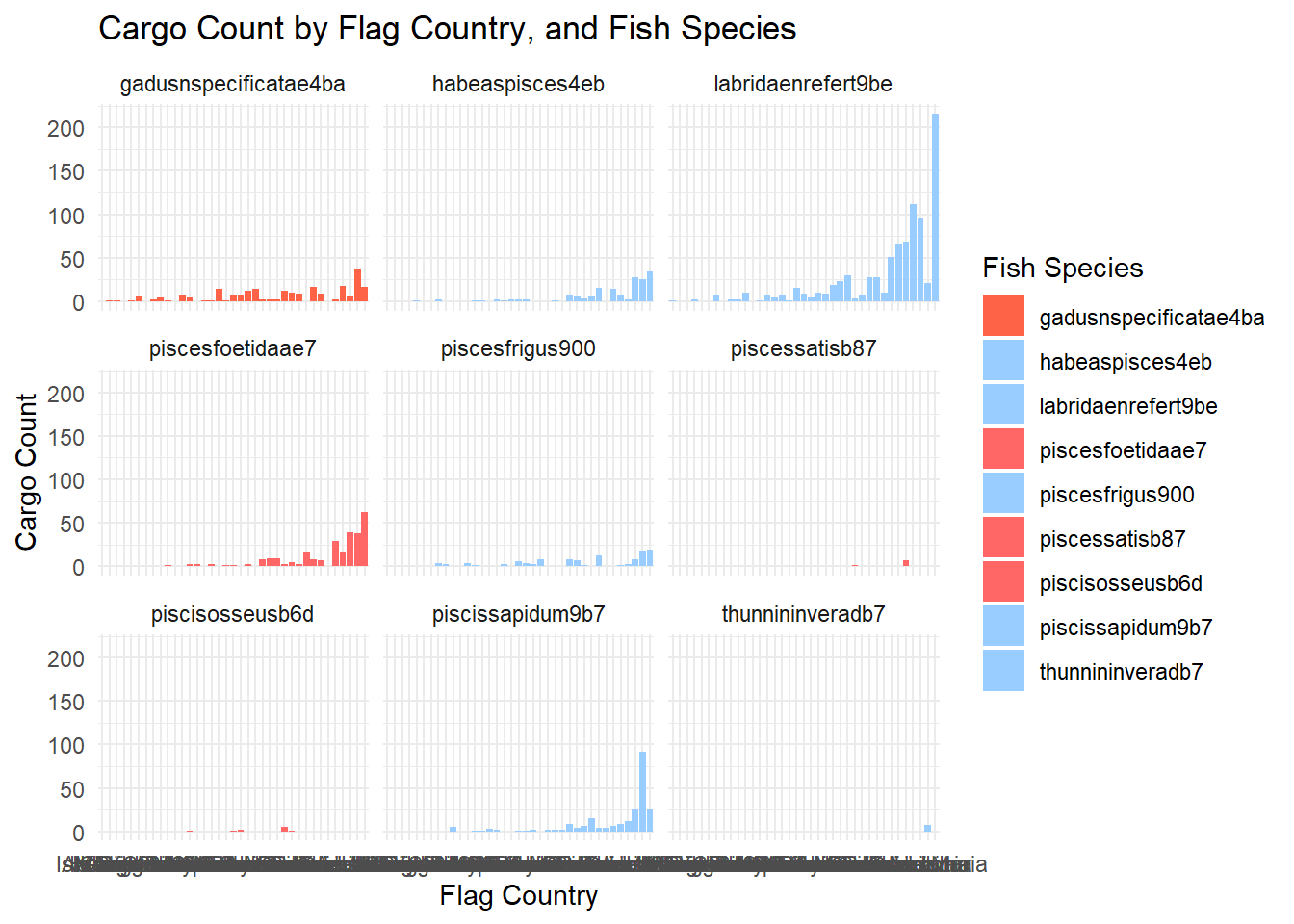

Zooming into cargo vessels with illegal fish species, we observe the months which they are delivered

Code

non_fishing_illegal_match <- mapped_records %>% 
  filter(vessel_type != "Fishing", 
         fish_species %in% c("piscisosseusb6d", "piscessatisb87", "gadusnspecificatae4ba"))

unique(non_fishing_illegal_match$vessel_id) #35 distinct vessel ids

 [1] "seasphere38e"         "transpacific5ada"     "maritimematrix7755"  
 [4] "harborhelios585"      "freightfusion141"     "nauticalnirvana874"  
 [7] "cargocentric4d0"      "transatlantic77d"     "blueharbor2c1"       
[10] "nauticalnexus1a5d"    "freightfrontiers7134" "maritimemomentumfab" 
[13] "vesselvanguard5d06"   "maritimemover13f"     "oceanicoasisd3f"     
[16] "seasystem3e22"        "vesselvictoryafd"     "seawayspectra490"    
[19] "aquatransit6bc"       "seasentinel24e"       "oceanicoracle9da"    
[22] "maritimemiraclef85"   "maritimemagnitude2e9" "harborhalo9dd6"      
[25] "transoceane48"        "seasolutions4d5"      "transcontinentalcf3" 
[28] "oceanicline3de"       "seawayspectrumca2"    "seasystem375"        
[31] "harborhavenf91"       "nauticalnexus6cc"     "cargocynosure29d"    
[34] "seasentry2e28"        "vesselvistad0c"

Code

unique(non_fishing_illegal_match$flag_country) # 30 distinct countries

 [1] "Orvietola"       "Arreciviento"    "Alverossia"      "Lumakari"       
 [5] "Solovarossa"     "Rio Solovia"     "Lumindoria"      "Luminkind"      
 [9] "Mawalara"        "Riodelsol"       "Azurionix"       "Playa Solis"    
[13] "Khamseena"       "Brindisola"      "Kethanor"        "Nalaloria"      
[17] "Oceanus"         "Korvelonia"      "Ariuzima"        "Coralmarica"    
[21] "Gavanovia"       "Calabrand"       "Yggdrasonia"     "Nyxonix"        
[25] "Isla Solmar"     "Thessalandia"    "Utoporiana"      "Islavaria"      
[29] "Kuzalanda"       "Anderia del Mar"

Code

# loading packages for parallel plots
pacman::p_load(GGally, parallelPlot)

# summarizing cargo records into month

non_fishing_illegal_match_summary <- non_fishing_illegal_match %>%
  mutate(month = floor_date(tx_date, "month")) %>%
  group_by(dest, month, fish_species) %>%
  summarise(total_qty_tons = sum(qty_tons), 
            vessel_count = n_distinct(vessel_id)) %>%
  ungroup()

# plotting the summary over month 
ggplot(non_fishing_illegal_match_summary, aes(x = month, y = total_qty_tons, color = fish_species, group = fish_species)) +
  geom_line() +
  geom_point() +
  labs(x = "Month", y = "Total Cargo Quantity (tons)", title = "Cargo Quantity Over Time by Destination and Fish Species") +
  facet_wrap(~ dest, ncol = 1) +
  scale_fill_manual(values = species_colors) +  
  theme_minimal() +
  scale_x_date(date_labels = "%b %Y", date_breaks = "1 month") +
  theme(axis.text.x = element_text(angle = 45, hjust = 1))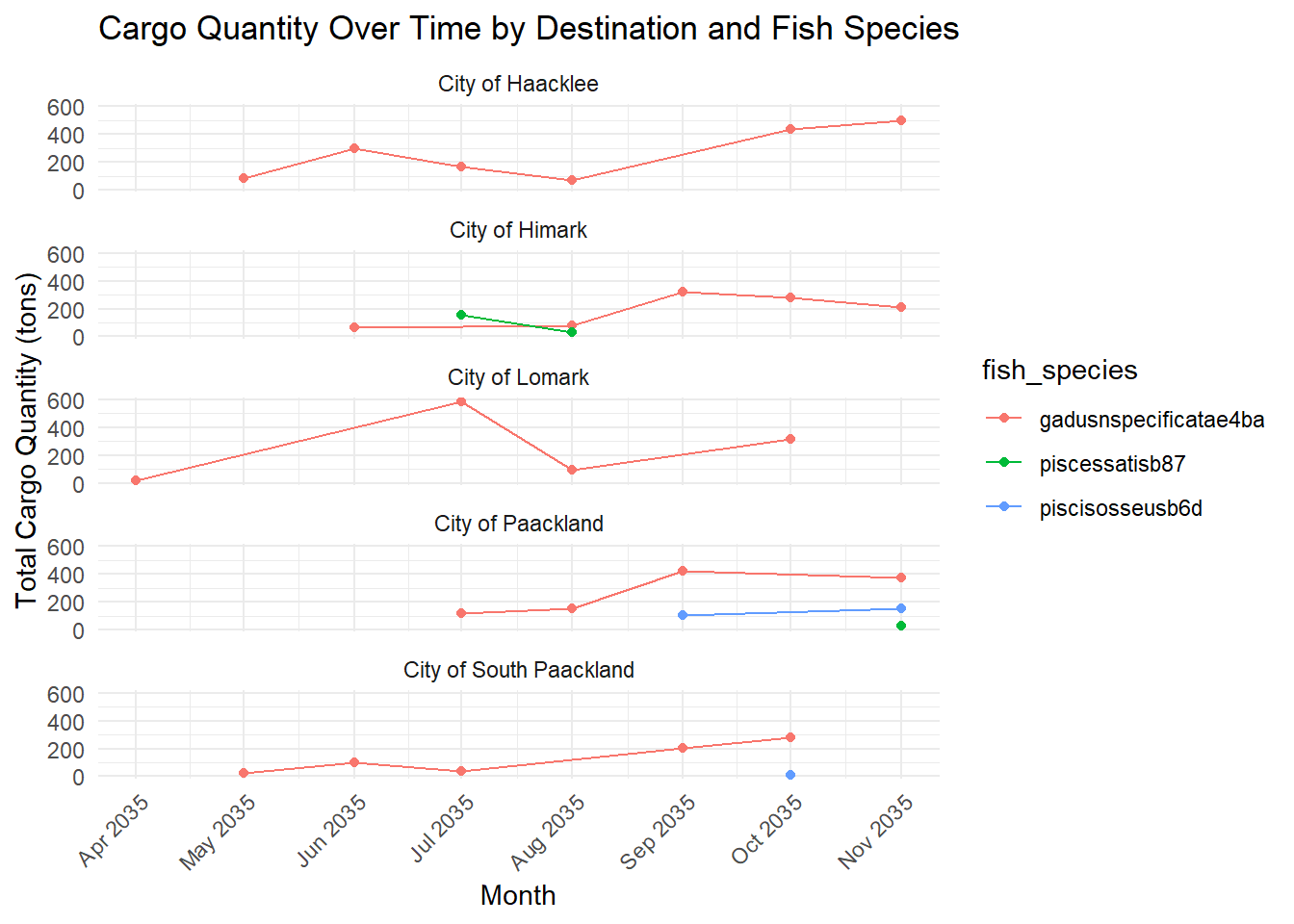

Contrasting with the cargo data (full population)

Code

tx_qty$tx_date <- as.Date(tx_qty$tx_date)

tx_by_mth <- tx_qty %>%
  mutate(month = floor_date(tx_date, "month")) %>%
  group_by(dest, month, fish_species) %>%
  summarise(total_qty_tons = sum(qty_tons))

# fish species color with salmon 
species_colors <- c(
  "gadusnspecificatae4ba" = "#FF6666",  # Illegal
  "habeaspisces4eb" = "#99CCFF",        # Legal
  "labridaenrefert9be" = "#99CCFF",     # Legal
  "piscesfoetidaae7" = "#FF6666",       # Illegal
  "piscesfrigus900" = "#99CCFF",        # Legal
  "piscessatisb87" = "#FF6666",         # Illegal
  "piscisosseusb6d" = "#FF6666",        # Illegal
  "piscissapidum9b7" = "#99CCFF",       # Legal
  "thunnininveradb7" = "#99CCFF",       # Legal
  "oncorhynchusrosea790" = "#FFFF99"    # Salmon
)

## plot
ggplot(tx_by_mth, aes(x = month, y = total_qty_tons, color = fish_species, group = fish_species)) +
  geom_line() +
  geom_point() +
  labs(x = "Month", y = "Total Cargo Quantity (tons)", title = "Cargo Quantity Over Time by Destination and Fish Species") +
  facet_wrap(~ dest, ncol = 1, strip.position = "left") +
  scale_color_manual(values = species_colors) +  
  theme_minimal() +
  scale_x_date(date_labels = "%b %Y", date_breaks = "1 month") +
  theme(
    axis.text.x = element_text(angle = 45, hjust = 1),
    strip.placement = "outside",
    strip.text.y.left = element_text(angle = 0),  # Rotate facet labels
    panel.spacing = unit(1, "lines")  # Increase space between panels
  ) +
  coord_cartesian(clip = "off")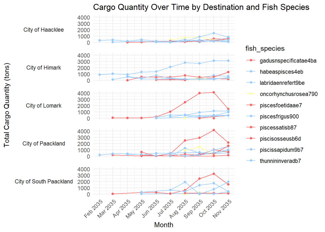

Comparing with the cargo mapped to suspicious vessel for South Seafood Corp

10 cargo mapped
Summary only to 2 ports, of 2 months

Code

ss_cargo <- mapped_records %>% 
  filter(vessel_id %in% c("snappersnatcher7be", "roachrobberdb6"))

# formatting to align with tx_by_month dataframe 

ss_by_month <- ss_cargo %>%
  mutate(month = floor_date(tx_date, "month")) %>%
  group_by(dest, month, fish_species) %>%
  summarise(total_qty_tons = sum(qty_tons))

ggplot(tx_by_mth, aes(x = month, y = total_qty_tons, color = fish_species, group = fish_species)) +
  geom_line() +
  geom_point() +
  geom_point(data = ss_by_month, aes(x = month, y = total_qty_tons), color = "purple", size = 1) +  # Highlight points in purple
  labs(x = "Month", y = "Total Cargo Quantity (tons)", title = "Cargo Quantity Over Time by Destination and Fish Species") +
  facet_wrap(~ dest, ncol = 1, strip.position = "left") +
  scale_color_manual(values = species_colors) +  
  theme_minimal() +
  scale_x_date(date_labels = "%b %Y", date_breaks = "1 month") +
  theme(
    axis.text.x = element_text(angle = 45, hjust = 1),
    strip.placement = "outside",
    strip.text.y.left = element_text(angle = 0),  # Rotate facet labels
    panel.spacing = unit(1, "lines")  # Increase space between panels
  ) +
  coord_cartesian(clip = "off")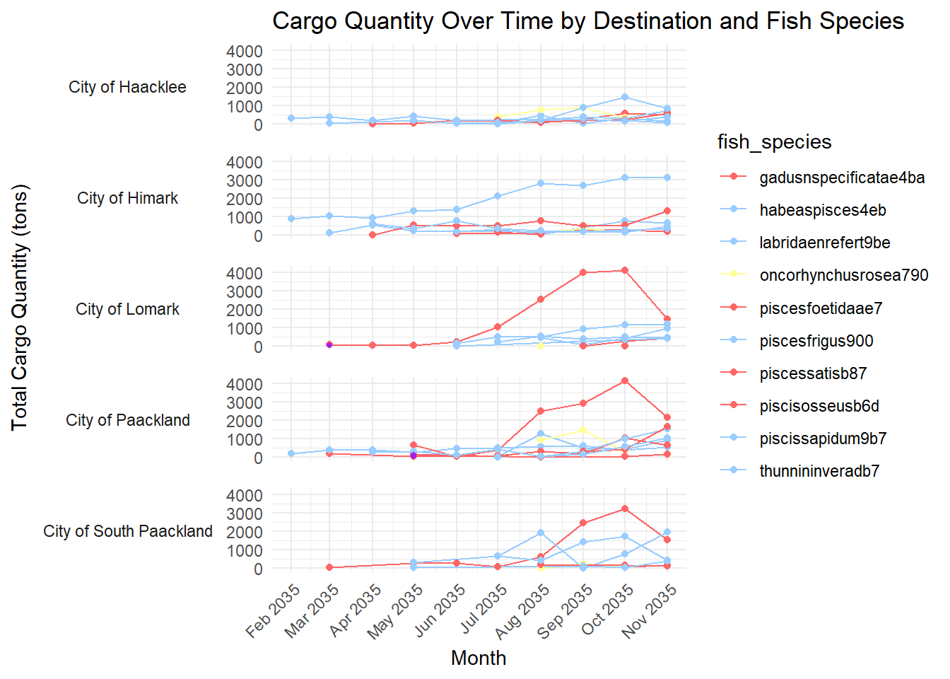

Comparing with vessels of similar size to South Seafood Corp vessels.

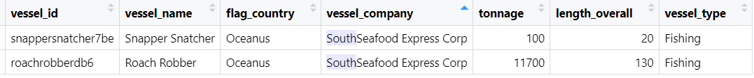
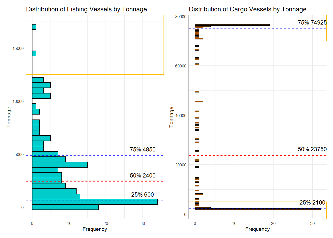
Introducing filter to identify vessels of certain tonnage.

9 other small fishing vessels of <= 100 tonnage similar to Snapper Snatcher
7 other large vessels of >= 11700 tonnage similar to Roach Robber
Issue: No linked cargo to Roach Robber

Code

ss_vessel <- N_vessel %>% filter(vessel_company %in% "SouthSeafood Express Corp")

# Returning vessels that are unusually small like Snapper Snatcher

sus_small_tonnage <- 100
sus_small_vessels <- N_vessel %>% 
  filter(tonnage <= sus_small_tonnage, vessel_type == "Fishing") %>% 
  mutate(sus_type = "abnormally_small")

# Returning vessels that are unusually large like Roach Robber

sus_large_tonnage <- 11700
sus_large_vessels <- N_vessel %>% 
  filter(tonnage >= sus_large_tonnage, vessel_type == "Fishing") %>% 
  mutate(sus_type = "abnormally_large")

sus_size_fish_vessel <- rbind(sus_small_vessels, sus_large_vessels)

# identifying matching cargo for small vessels 

sus_size_vessels_cargo <- mapped_records %>% 
  filter(vessel_id %in% sus_size_fish_vessel$vessel_id) %>%
  left_join(sus_size_fish_vessel %>% 
              select(vessel_id, sus_type), by = c("vessel_id" = "vessel_id"))

#write_csv(sus_size_vessels_cargo, "data/sus_vessel_cargo.csv")

sus_size_vessels_cargo_summary <- sus_size_vessels_cargo %>%
  group_by(vessel_id, dest, sus_type) %>%
  summarize(median_qty_tons = median(qty_tons, na.rm = TRUE)) %>%
  ungroup()

# Create the parallel coordinates plot
data_wide <- sus_size_vessels_cargo_summary %>%
  pivot_wider(names_from = dest, values_from = median_qty_tons) %>%
  replace(is.na(.), 0)

# Assigning color for South Seafood vessels 
vessel_colors <- c("snappersnatcher7be" = "#FF6666", 
                    "roachrobberdb6" = "#FF6666", 
                   "default" = "grey") 

# Create a color column based on vessel_id
data_wide$color <- ifelse(data_wide$vessel_id %in% names(vessel_colors),
                          vessel_colors[data_wide$vessel_id],
                          vessel_colors["default"])

# Create the parallel coordinates plot with facet wrap for sus_type
ggparcoord(data = data_wide, 
           columns = 3:ncol(data_wide), # Columns for median_qty_tons
           groupColumn = 1, # Column index for vessel_id
           scale = "globalminmax",
           alphaLines = 0.5, 
           boxplot = TRUE) +
  scale_color_manual(values = vessel_colors) + 
  labs(title = "Parallel Coordinates Plot of Vessel Cargo Data",
       x = "Port",
       y = "Median Quantity in Tons",
       color = "Vessel ID") +
  theme_minimal() +
  facet_wrap(~ sus_type, ncol = 1)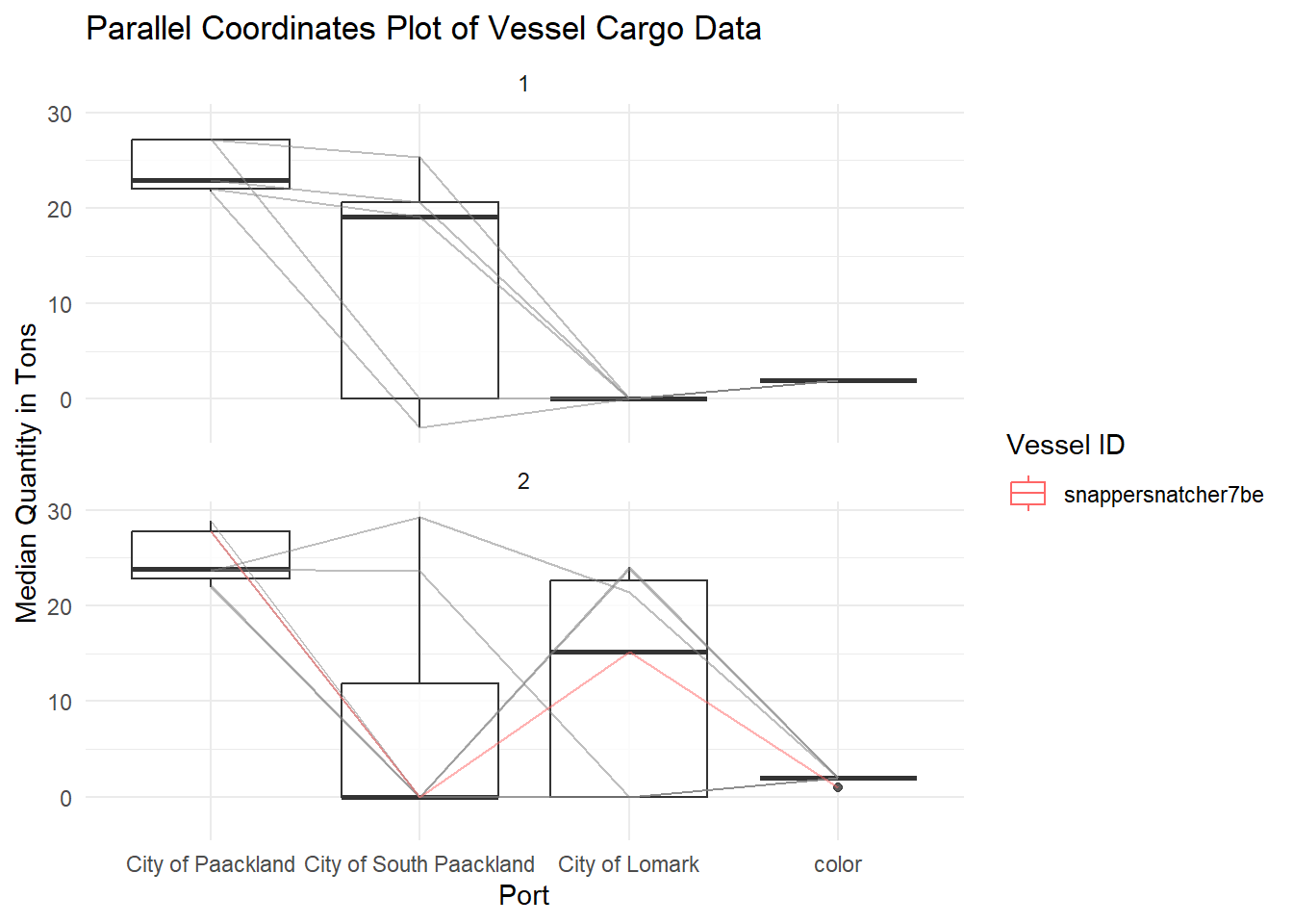

Creating parallel plot for median fish quantity cargo declared at each port.

Code

# summarizing median cargo qty 
vessels_cargo_summary <- mapped_records %>%
  mutate(month = floor_date(tx_date, "month")) %>%
  group_by(vessel_id, dest, fish_species, month) %>%
  summarize(median_qty_tons = median(qty_tons, na.rm = TRUE)) %>%
  ungroup()


# filter of destination of interest
vessel_cargo_summary_paackland <- vessels_cargo_summary %>% 
  filter(dest == "City of Paackland")

# converting to format for plot
data_wide <- vessel_cargo_summary_paackland %>%
  pivot_wider(names_from = month, values_from = median_qty_tons) 

# scatter plot 
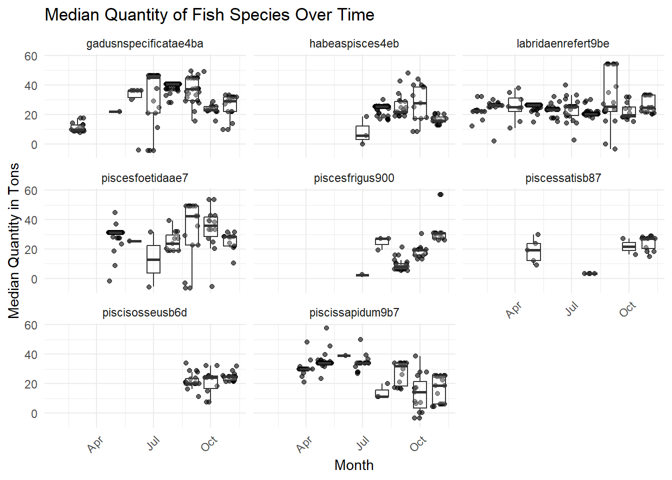
ggplot(vessel_cargo_summary_paackland, aes(x = month, y = median_qty_tons)) +
  geom_jitter(alpha = 0.6) + # Scatter plot with jitter for each vessel
  geom_boxplot(aes(group = month), alpha = 0.3, outlier.shape = NA) + # Box plot
  labs(title = "Median Quantity of Fish Species Over Time",
       x = "Month",
       y = "Median Quantity in Tons") +
  facet_wrap(~ fish_species) + 
  theme_minimal() +
  theme(axis.text.x = element_text(angle = 45, hjust = 1))